Beyond PulseSync: Less Clock Granularity Impact,
More Synchronization Accuracy
Xiaoyuan Ma, Weisheng Tang, Jianming Wei, Jun Huang and Bo Zhang
Shanghai Advanced Research Institute, Chinese Academy of Sciences, Haike Road, Shanghai, China
Keywords:
Clock Synchronization, WSN, Clock Granularity, PulseSync.
Abstract:
Nowadays clock synchronization has become crucial in wireless sensor network (WSN), in particular for
those scenarios where the common reference time is vital for applications. The existing approaches often
suffer from synchronizing errors since the effect of clock granularity is overlooked. In this paper, a novel
algorithm is proposed on the basis of PulseSync algorithm. Compared with PulseSync, the improvement of
the presented algorithm is twofold: First, clock discreteness is abated via applying filter method. Second, for
reducing the deviation of estimated clock skew through several hops, relative logical clock rate is straightly
delivered. Our approach, along with the deeper analyses, is further validated with EXP5438 platform using
Contiki operating system in Cooja simulator. The result illustrates that the proposed algorithm outperforms
PulseSync in synchronization accuracy.
1 INTRODUCTION
Recently, WSN has been applied in a wide range
of fields including environment monitoring, object
detecting, military supervisory, precision agriculture
and so forth(Martinez et al., 2004). Its high popu-
larity is due to great boosts in related technologies
such as electronics, Micro-electromechanical sys-
tem (MEMS), wireless communication, etc. Simply
put, WSN is essentially a distributed network sys-
tem where a huge number of nodes are densely de-
ployed and communicate with each other via multi-
hops mechanism.
One of the most key issues in WSN is time syn-
chronization which plays a very important role in a
bunch of related technologies from node energy man-
agement mechanism to Media Access Control (MAC)
based on time slots(Cionca et al., 2008). Abundant
applications are also highly dependent on time syn-
chronization in which a common time scalar could
be obtained by nodes communicating with each other
and adjusted by themselves. Therefore, many re-
searches are focused on the aspect of WSN time syn-
chronization in these years.
Time synchronization in WSN is confronted with
greater challenges than those center-based time syn-
chronization systems such as GPS and Network Time
Protocol-based (NTP)(Mills et al., 2010)x. Above all,
nodes in WSN play two roles: sender and receiver,
which means that each node brings its own time into
correspondence with its predecessor and meanwhile
delivers or broadcasts the reference time to succes-
sors. Secondly, the node’s process capability gets
limited in consideration of the need of low cost and
power consumptions in WSN applications. Lastly,
time synchronization also need to take account into
mobility, crystal frequency drift caused by environ-
mental factors and other constraints.
This paper proposed an improved time synchro-
nization algorithm which originates from PulseSync
algorithm(Lenzen et al., 2009; Lenzen et al., 2014).
The proposed algorithm is superior to PulseSync in
that the impact of clock granularity has been taken
into account to deal with synchronization error in-
duced by multihops of communication. Similar to our
method, Virtual High-resolutionTime (VHT)(Schmid
et al., 2010) also is oriented towards the issue of the
clock granularity. But different from VHT, no extra
hardware device/resource is required by ours.
Usually, the skew estimation is affected by the
clock granularity in PulseSync and some other tradi-
tional WSN synchronization algorithms or protocols.
To overcome the problem, two main contributions are
achieved in this paper:
Firstly, statistic filter method is imposed on rel-
ative logical clock rate to abate the impact of dis-
creteness of clock value.
Owing to the space distance among adjacent
Ma, X., Tang, W., Wei, J., Huang, J. and Zhang, B.
Beyond PulseSync: Less Clock Granularity Impact, More Synchronization Accuracy.
DOI: 10.5220/0005632600950104
In Proceedings of the 5th International Confererence on Sensor Networks (SENSORNETS 2016), pages 95-104
ISBN: 978-989-758-169-4
Copyright
c
 2016 by SCITEPRESS – Science and Technology Publications, Lda. All rights reserved
95

nodes is not far, vicinage nodes are assumed to be in
the same circumstance and those crystal drift is grad-
ual and continuous. Statistical filter such as Kalman
filter is invoked to make the deviation of the relative
logical clock rate less.
Secondly, the relative logical clock rate besides
the clock value is delivered straightly to mitigate
the deviation of the estimated clock skew.
The approach that estimated clock skew computed
with clock value in common algorithms will be af-
fected by the clock granularity naturally. On the con-
trary, relative logical clock rate can be expressed more
precisely in the same bit width and the deviation of
estimated clock skew will decrease as a result.
The organization of this paper is as follows: the
related researches will be reviewed in Section 2. In
Section 3, we shall describe PulseSync concisely and
deep into the clock granularity effects. The improved
method is proposed in Section 4. In Section 5, the
results of simulation and some remarks are provided.
We draw conclusion in Section 6.
2 RELATED WORK
In the past decades, there have been numerous re-
searches on WSN time synchronization protocol.
Timing-sync Protocol for Sensor Networks
(TPSN)(Ganeriwal et al., 2003) is a classical
sender-receiver synchronization (SRS) method.
The synchronizing packet containing timestamps
needs to be exchanged between two nodes in
TPSN. One category of the criticisms about TPSN
is neglecting the estimation of clock skew, and
the other is its requirement of frequent commu-
nication. In order to overcome the first sort of
drawback, TINY-SYNC/MINI-SYNC(Sichitiu and
Veerarittiphan, 2003) was raised where the clock
skew estimation was taken into consideration.
However, the second of the issues was solved by
another kind of synchronization method named
Receiver-receiver synchronization (RRS). Reference
Broadcast Synchronization (RBS)(Elson et al., 2002)
is one representative case where two receivers get
timing packet from one broadcast beacon. Once
obtained the packet, receivers record timestamps in
accordance with their local clocks. Furthermore,
the two receivers also communicate with each other
for calculating the relative skew using least-squares
linear regression. The great advantage of RBS is its
capability of eliminating the time of the transmission
and the media access. Although its success in time
synchronization, RBS still gets stuck in tackling with
those non-deterministic time delays in transmission,
media access and receiving procedure. Concerned
with the above problems, M.Maroti et al (Mar´oti
et al., 2004) put forward flooding Time Synchro-
nization Protocol (FTSP) in which the operation of
timestamping is moved down to the MAC layer and
results in reduction of non-deterministic access time.
In addition, FTSP decreases the communication
frequency and makes that less than RBS.
Nowadays, researchers have paid more attentions
to alleviating time synchronization errors in real net-
work, especially in multihops communication sce-
nario. They observed that neighbor nodes in practical
WSN may communicate at short intervals or collab-
orate on executing a common task while the distant
nodes seldom exchange the information. Motivated
by the phenomenon, numerous improved approaches
have been raised. For instance, Nancy Lynch et al
proposed Gradient Clock Synchronization (GCS) the-
oretically in (Fan and Lynch, 2006). On the basis of
GCS, Philipp Sommer et al implemented the Grandi-
ent Time Synchronization Protocol (GTSP)(Sommer
and Wattenhofer, 2009) where the estimated logical
clock skew of each node tends to be a constant un-
der the circumstance of strong connection. In or-
der to synchronize with the neighbor nodes precisely
in GTSP, each node will increase their logical clock
skew by averaging skew among neighboring clocks.
The fully distributed synchronization algorithms, e.g.
GTSP, could be an approach to solving the problem of
synchronization error accumulation in multi-hop net-
work via achieving less time error in neighbor nodes,
yet GTSP yields the more global time error.
Unlike GTSP, Lenzen et al.(Lenzen et al., 2009)
proposed an alternative to lessen time synchroniza-
tion errors resulting from multihops. In (Lenzen
et al., 2009), time synchronizationerror was analyzed.
More importantly, the authors pointed out the reason
why FTSP yields time synchronization error via mul-
tihops and then proposed PulseSync algorithm. The
essential idea of PulseSync is to align the delivery
of synchronization packets in each node. This ap-
proach increased the accuracy between two nodes that
are not adjacent by minimizing the estimated error of
multihops-induced skew.
After PulseSync, there also have been significant
advances in clock synchronization, especially from
signal processing perspectives(Duand Wu, 2013; Luo
and Wu, 2013; Wu et al., 2011). But most of them
disregarded the clock granularity that may be princi-
pal factor of the error sometimes except that the Vir-
tual High-resolution Time (VHT) was presented in
(Schmid et al., 2010) to refine the clock granularity
with one extra hardware interrupt or logical device,
e.g. FPGA. Nevertheless, the hardware interrupt re-
SENSORNETS 2016 - 5th International Conference on Sensor Networks
96

sources on the MCU chip is inadequate generally and
it is almost impossible to be equipped with FPGA in
nodes in many rigor applications due to the limitation
of power consumption and physical size. Thus, it is
quite necessary to regard the clock value discreteness
without any extra hardware resources and the impact
of clock granularity will be analyzed in Section 3.
3 ANALYSIS
In this part, the models and several notations used in
this paper will be introduced in 3.1. Then, we shall
analyze the multihops-produced error because of the
clock granularity in 3.2.
3.1 Models
Individual Node
Typical clock on a WSN node consists of a crystal
oscillator and a counter. The counter will decrease
when the crystal oscillator oscillates once. An in-
terrupt will be triggered and the counter resets when
the counter decrease to zerox. The logical clock (an-
other clock) increases in the interrupt service rou-
tines (ISR). The application programs on WSN node
read and utilize the logical clock value through the
application-programming interface (API).
Given the rate of crystal oscillator h(t), the hard-
ware clock H
i
(t) of node i is computed as follows:
H
i
(t) =
Z
t
t
0
h
i
(τ)dτ + Φ
i
(t
0
) (1)
where Φ
i
(t
0
) is the hardware clock offset at time t
0
.
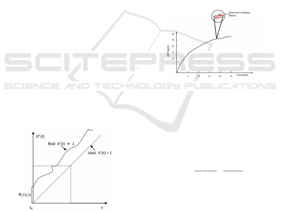
Figure 1: Rate of crystal oscillator.
As shown in Figure 1, ideally, h
i
(t) ought to be
constant whose value is one (like the slope of the dot-
ted line). But practical crystals will not be same ex-
actly and many outside elements such as environmen-
tal temperature, power supply voltage and aging (Vig,
2001) probably cause the frequency drift, so h
i
(t) is
not an constant, i.e.,
h
i
(t) ∈ [1 −ρ, 1+ ρ] (2)
where ρ is the maximum frequency tolerance of
the crystal that often can be referred to the related
datasheet. Normally, the range of ρ is 1 to 100ppm.
WSN node is unable to adjust the hardware clock
H
i
(t) by itself but the logical clock can be corrected.
It is calculated as follows:
L
i
(t) =
Z
t
t
0
h
i
(τ)l
i
(τ)dτ + Ψ
i
(t
0
) (3)
where L
i
(t) is the logical clock of node i. l
i
(t) is the
relative logical clock rate. Ψ
i
(t
0
) is the offset between
the logical clock and the hardware clock on node i at
time t
0
.
Discussions about h(t)
Figure 2: Aging and short-term stability(Vig, 2001).
Besides drift, short-term instability of crystal os-
cillator is more nondeterministic. According to (Vig,
2001), as illustrated in Figure 2, drift is a kind of ef-
fect that is observed over long periods of time (hours,
days or years), whereas the other is random and ob-
served over periods that are typically measured in
fractions of a second to minutes. The instantaneous
frequency h(t) of the practical crystal oscillator with
noise can be expressed as(Stein, 1985),
h(t) = h
c
(t) +
1
2π
dφ(t)
dt
,




φ(t)
2πh
c
(t)




≪ 1 (4)
where the current frequency of crystal oscillator h
c
(t)
can be regarded as constant h
c
since it drifts with
time slowly. The deviation of phase from the ideal
is φ(t). Generally, φ(t) consists of white and flicker
noises taking the form of phase jitters which may re-
flect jitters of message. The goal of time synchroniza-
tion is to share identical time scale through achiev-
ing the same clock skews h(t) ·l(t) and proper off-
sets Ψ
i
(t
0
). The clock skews are designed to compen-
sate the drift rather than stochastic short-term instabil-
ity. Conversely, skews estimation can be worsened by
Beyond PulseSync: Less Clock Granularity Impact, More Synchronization Accuracy
97

both jitters and clock granularity. The latter is stated
in Clock Granularity of 3.2.
Nodes in Network
Time synchronization in large-scale WSN is one of
the many challenges. Multihops between nodes and
the root node(reference) become another factor de-
grading the precision of skews estimation. Thus mul-
tihops scenario is considered. For simplicity, given
three nodes i−1, i and i+1 in link-like topology, node
i received messages from the predecessor node i −1
and synchronize to it. The similar processes occur be-
tween node i and its successor i+ 1. The distance be-
tween two nodes is defined as the hops. For instance,
the distance that is denoted as d between node 2 and
node 5 is three.
The ultimate goal of time synchronization in one
network with n nodes is that all the logical clocks and
all the clock skews h(t)·l(t) are both identical at time
t.

L
1
(t) = L
2
(t) = ... = L
n
(t)
h
1
(t) ·l
1
(t)=h
2
(t) ·l
2
(t)=.. .=h
n
(t) ·l
n
(t)
(5)
Generally, there is only one root node r in the net-
work to which all the others synchronize themselves.
Thereupon, Equations (5) can be re-written more pre-
cisely as follows:







L
1
(t) = L
2
(t) = ... = L
n
(t)
h
1
(t) ·l
1→r
(t)
=h
2
(t)·l
2→r
(t)= ... =h
n
(t)·l
n→r
(t)= h
r
(t)
(6)
where, for node n, l
n→r
(t) is relative logical clock
rate to the root node r.
Multihops error that is induced by clock granular-
ity will be discussed below.
3.2 Multihops Error
First of all, some conclusions in (Lenzen et al., 2009)
will be described here.
3.2.1 About PulseSync
According to (Lenzen et al., 2009), in the case of
d = 1, the probability that relative logical clock rate
ˆ
l
i→r
(t) computed by node i has an error of at least
Ω( j/Bk
3/2
) is constant:
P



ˆ
l
i→r
(t) −l
i→r
(t)


≥ Ω

j
Bk
3/2

≥
1
2
(7)
where B is the PulseSync’s synchronization periods.
The jitter of messages meets the Gaussian Distribu-
tion
1
with a standard deviation j or uniformly dis-
tributed in [−j, j]. Each node estimates the logical
relative rate based on k observation values.
ˆ
l
i→r
(t) is
estimated by node i and l
i→r
(t) is the real value. For
better description, j/Bk
3/2
is denoted as E( j).
When d > 1, the error of relative logical clock rate
ˆ
l
i→r
(t) on node i is,
E( j) =
j
√
d
Bk
3/2
(8)
The lower bound (the maximum difference of log-
ical clock value between any two nodes) of PulseSync
is as follows:
G(t) ∈ Ω

j
√
D
√
k

(9)
where D is the diameter of the network N. The ef-
fect of clock granularity ignored in PulseSync(Lenzen
et al., 2009) will be delved below.
3.2.2 Clock Granularity
In practice, the clock value of WSN node is discrete.
When receiving two identical clock values, the node
hardly makes a distinction between them and brings
quantization error that will be amplified through mul-
tihops as with the message jitter. Multihops error is
composed of message jitter and clock granularity.
Therefore, the jitter should be represented as fol-
lows:

T
jitter
T
gran

·T
gran
+ υ·T
gran
(10)
where T
gran
is clock granularity and suppose that υ
is a Bernoulli distributed random variable with mean
of 0.5. T
jitter
is the time of jitter. ⌈·⌉ is the symbol
of rounding-up. Consequently, when considering the
discreteness of t, E( j) could be represented as fol-
lows:
E( j) =

⌈
j
T
gran
⌉+ 0.5

·T
gran
Bk
3/2
(11)
Similarly, like Equation (8), E( j) is as follows on
the condition of d > 1:
E( j) =
√
d ·

⌈
j
T
gran
⌉+ 0.5

·T
gran
Bk
3/2
(12)
where

⌈
j
T
gran
⌉+0.5

·T
gran
Bk
3/2
is denoted as γ( j).
1
Jitter is not exactly Gaussian Distribution, but we can
make it zero mean and the resulting behavior is very similar.
SENSORNETS 2016 - 5th International Conference on Sensor Networks
98

As a result, in practice, the lower bound of Puls-
eSync should be as follows:
G(t) ∈ Ω(
√
Dγ( j)Bk) (13)
Equation (11) shows two points:
a) γ( j) will exists even though j is minor enough
to be ignored;
b) If T
gran
is small enough, γ( j) ≈ j; on the other
hand, if T
gran
≫ j, the numerator of γ( j) is governed
by T
gran
.
The first point indicates that the error of relative
logical rate estimation will exists even though j tends
to zero. The second implies that jitters j can be
regarded as γ( j) when the clock resolution is high
enough. Conversely, clock granularity will take on
a more dominant factor and can not be neglected any
more as it is coarser. It is worth noting that, some-
times, the errors in real time (not in clock ticks) will
significantly reduce the synchronization accuracy due
to the coarse clock granularity. Equation (12) means
that the multihops error cannot be annihilated in Puls-
eSync as long as t is discrete. The clock granularity
T
gran
dominates the synchronization error in that mul-
tihops synchronization error exists even if the jitter
tends to zero.
Equation (11) suggests that E( j) is proportional to
T
gran
. However, generally speaking, reducing clock
granularity indicates increasing operating frequency
and leading to significant amount of node’s power
consumption as a result. In contrast, this paper argue
that the clock granularity impact could be relieved by
filtering and delivering the relative logical clock rate
without changing T
gran
.
4 IMPROVED PULSESYNC
The improvements are presented in this section. We
describe the main idea of the algorithm in 4.1 and do
some explanations concerning the filter in 4.2.
4.1 Algorithm Description
Figure 3: Synchronization message flow diagram.
In general, for one node, the process of synchroniza-
tion needs to estimate the relative logical clock rate
and the offset between itself and the root node that
is the reference. In the algorithm, the offset value
Ψ
i
(t
0
) of node i in Equation (3) is obtained in the
same way as PulseSync. With the purpose of abating
the impact of the clock granularity,the work is mainly
devoted to getting the relative logical rate improved
throughout four steps. Nodes are arranged as link
topology and messages flow as Figure 3. Each node
regards the root node as the only reference. L
r
(t
q
)
ought to become the global clock as all the nodes
in the network synchronizing successfully. Message
{1,H
r
(t
q
),L
r
(t
q
),q} with the sequence number q is
broadcasted by the root node at time t
q
. Then it is re-
ceived by node i at time t
q
+ δ. δ
µ
is very small since
node i delivers it promptly at time t
q
+ δ + δ
µ
once
receiving the qth message.
The main procedures of the algorithm will be
stated below.
Step 1:
Node i refreshes
ˆ
l
i→i−1
(t
q
+ δ) and
Ψ
i
(t
q
+ δ) once receiving message.
When receiving the synchronization message
from node i−1, node i calculates
ˆ
l
i→i−1
(t
q
+ δ) using
H
i−1
(t
q
+ δ) contained in the packet and Ψ
i
(t
q
+ δ)
through L
i−1
(t
q
+ δ). Therefore,
h
i−1
(t
q
+ δ) = h
i
(t
q
+ δ) ·
ˆ
l
i→i−1
(t
q
+ δ) (14)
Step 2:
Node i smooths
ˆ
l
i→i−1
.
Node i gets
¯
l
i→i−1
(t
q
+ δ) as the result of smooth-
ing
ˆ
l
i→i−1
(t
q
+ δ) with Kalman Filter.
Step 3:
Node i calculates
ˆ
l
i→r
(t
q
+ δ).
ˆ
l
i→r
(t
q
+ δ) can be get as the following:
ˆ
l
i→r
=
ˆ
l
i−1→r
·
¯
l
i→i−1
(15)
where
¯
l
i→i−1
·h
i
= h
i−1
. If the distance between node
i and root node r is d,
ˆ
l
i→r
is boiled down to product
of all relative logical clock rates on the routine from r
to i, i.e.,
ˆ
l
i→r
=

d
∏
n=2
¯
l
n→n−1

·(
ˆ
l
1→r
) (16)
Step 4:
Node i encapsulates {
ˆ
l
i→r
(t
q
+ δ +
δ
µ
),H
i
(t
q
+ δ+ δ
µ
),L
i
(t
q
+ δ+ δ
µ
),q} and delivers it.
It is noted that
ˆ
l
i→r
(t
q
+ δ + δ
µ
) is equivalent to
ˆ
l
i→r
(t
q
+δ) since the time δ
µ
is quite short. According
to the Equation (3), L
i
(t) can be written as follows:
L
i
(t)
=
R
t
t
q
+δ
h
i
(τ)·
ˆ
l
i→r
(t
q
+δ)dτ+Ψ
i
(t
q
+δ),t>t
q
+δ
(17)
The pseudo-code is as follows (Figure 4). The
sequence number q is to avoid duplicated message
flooding in networks. On the root node, only broad-
casting reference messages and refreshing the se-
quence number q are required. Ordinary nodes check
Beyond PulseSync: Less Clock Granularity Impact, More Synchronization Accuracy
99

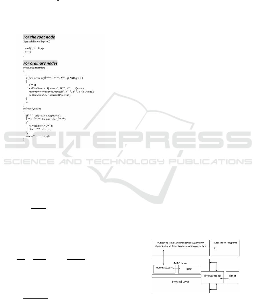
the sequence number q to ensure that the message is
new and maintain the Queue (a circular queue with
k-length) in the receiving interrupt service routine.
Function refresh is called to calculate psi and
ˆ
l
i→i−1
and accomplish sending when the receivingInterrupt
exits. Function RTimer
NOW returns the hardware
clock. In short, filtering improves the single-hop syn-
chronization performance and delivering relative log-
ical clock rates makes the filtering effect propagated
through multihops.
Figure 4: Pseudo-code of improved PulseSync.
4.2 The Reason of Utilizing Filter
As discussed in 3.1, the target of skews estimation in
time synchronization is to balance drifts, which is a
relatively gradual and continuous process, instead of
the short-term noises (jitters). For node i,
dh
i
(t)
dt
∈ [0−ς,0 + ς] (18)
where ς →0 and ς 6= 0. As Equation (14), the relation
between l
i+1→i
and h
i
is
h
i
= h
i+1
·l
i+1→i
(19)
If we differentiate equations (19) on both sides,
dh
i
dt
=
dh
i+1
dt
l
i+1→i
+
dl
i+1→i
dt
h
i+1
(20)
where both l
i+1→i
and h
i+1
tend to one. Therefore,
combined Equation (20) with (18), the change rate of
relative logical clock rate l
i+1→i
is
dl
i+1→i
(t)
dt
∈ [0−2ς,0+ 2ς] (21)
From Equation (21), l
i+1→i
is comparatively sta-
ble in very short time, motivating us to smooth out
the noise by statistics filtering. For instance, Kalman
filter is feasible. Detail model and parameters will be
expounded in Section 5.4.
So far, the improved algorithm has been proposed
and the next section will focus on implementation.
5 IMPLEMENTATION AND
SIMULATION
In this section, the simulation platform and imple-
mentation are delineated.
5.1 Simulation Platform
The simulation platform adopted in this paper is
Cooja Simulator(Eriksson et al., 2009). A simulated
Contiki Mote in COOJA executes Contiki(Dunkels
et al., 2004) operating system. Generally, the code for
specific platform could be easily ported to Motes in
Cooja without modifying for developers. EXP5438
platform is chosen as the mote in Cooja. The plat-
form EXP5438 is equipped with MSP430F5438 and
RF chip CC2420. The former is an ultra-low power
MCU with flash 256KB and RAM 16KB from Texas
Instruments. The latter is a packet-oriented RF chip
and the modulation mode is configured to FSK. The
system frequency of the EXP5438 is set to 8MHz by
multiplying the signal from a 32.768 kHz external
quartz crystal using a phased-locked loop. Also, the
crystal oscillator 32.768 kHz is used as the clock to be
synchronized. Moreover, in Cooja, the operating fre-
quency of all nodes is 7995492Hz actually and there
exists jitter of messages on every mote but no clock
drift. It is due to zero clock drift and same frequency
of all the nodes that the skew l
i→r
·h
i
is completely
dominated by the estimated relative logical clock rate
ˆ
l
i→r
.
5.2 Implementation in Contiki
Figure 5: The schematic diagram in Contiki.
According to Contiki, the time synchronization is
schemed as Figure 5. For reducing the communi-
SENSORNETS 2016 - 5th International Conference on Sensor Networks
100

cation overhead, the head of time synchronization
packet should be as short as possible. Hence, the com-
munication of time synchronization is completed in
MAC Layer, which brings synchronization indepen-
dent of the protocols (like TCP/IP) in upper layers.
In Contiki, exactly speaking, the timestamping
operation lying on the driver of RF eliminates the
stochastic MAC access time. In the CSMA mecha-
nism, when node sending packet, the node will per-
form the Clear Channel Assessment (CCA). If CCA
is valid and the packet with synchronization informa-
tion is ready to transmit (SFD pin is 1), the node will
timestamp in the packet. To avoid failure of writing
timestamps in time, some paddings are added to the
head. When receiving packet, node will not call the
corresponding ISR until the SFD is 1. Timestamping
executes in the ISR.
The synchronized logical clock will be provided
to applications in the form of API.
The hardware clock is 32.768KHz. It shows that
the clock granularity T
gran
is 1/32768 seconds. And
the waiting intervals before sending in both Puls-
eSync and the improved are set to zero.
5.3 Simulation
Figure 6: The topology in the simulation.
Since the algorithm in this paper is aimed to improve
the multihops error in time synchronization, chain
topology (Figure 6) is used to minimize the other in-
terferences. Each node can only communicate with
adjacent node in the chain topology (Figure 6). Node
1 is the root node which is the time reference.
Here, a testing node broadcasting packets in peri-
ods B is devised to facilitate evaluating the time syn-
chronization result. The requirement of testing node
is capable of covering all the nodes in the experiments
while denying replies to any common node in the net-
work. To cater for the demands and cut down work
loads, the testing node holds larger wireless cover-
age than other common nodes and disables receiv-
ing. Upon receiving the testing packet, the others will
timestamp and print the related information (includ-
ing estimated current relative logical clock rate to the
root node, the estimated current logical clock, etc.) to
the console of Cooja.
Moreover, 150 nodes (exclude testing node) are
deployed in totally and the network diameter D is 149.
Both the period of PulseSync and that of our algo-
rithm are all 20 seconds. The Radio Duty Cycling
(RDC) of all nodes is configured to ContikiMAC.
Broadcasting from testing node is scheduled between
two synchronization actions. The testing broadcast
period is also 20 seconds. To agree with practical sit-
uations, the rpl-collect application program is loaded
and run. The total length of simulation is 3 hours. The
main setups are collected in Table 1.
Table 1: Simulation Setups.
Network
Nodes number 150
Topology link
Running time 180mins
Nodes
Quartz crystal oscillator
frequency of nodes 32.768kHz
System frequency of nodes 8MHz
(using PLL from the crystal,
7995492Hz actually)
Operating System on nodes Contiki 2.6
MAC Layer(RDC) ContikiMAC(RDC)
MAC Layer CSMA
Applications running
while simulating rpl-collect
Synchronization
Beacon periods B 20s
Observation value number k 8
Hardware clock rate 32.768kHz
(no drifts but jitters exist
in this simulation)
Clock granularity 1/32768 s
Waiting time before sending 0
Smooth method Kalman filter
(2ς = 10
−9
, γ( j) = 10
−7
)
5.4 About the Kalman Filter
Combined with Equation (21), the process model of
the Kalman Filter can be represented as:

l
i→i−1
(t
m
) = l
i→i−1
(t
m−1
) + ω
m−1
l
i→i−1
obs
(t
m
) = l
i→i−1
(t
m
) + ϕ
m
(22)
where l
i→i−1
(t
m
) is the system state which denotes
the relative logical clock rate on node i at time t
m
.
l
i→i−1
obs
(t
m
) is the observation of the relative logical
clock rate on node i at time t
m
. The interval between
t
m
and t
m−1
stands for the synchronization periods
B. ϕ
m
is the noise produced by discreteness of clock
value, i.e.,
ϕ
m
∼ N (0, γ( j)) (23)
ω
m−1
is the process noise which is Gaussian dis-
tributed with standard deviation 2ς, i.e.,
ω
m−1
∼ N (0, 2ς) (24)
Beyond PulseSync: Less Clock Granularity Impact, More Synchronization Accuracy
101

In this simulation, 2ς is assumed to 10
−9
due to the
crystal drift is gradual and continuous when only af-
fected by environment. Moreover, taking the RAM
and communication ability into account, let k = 8,
B = 20s. In Figure 7, the standard deviation of es-
timated skew on node 2 with PulseSync (red curve) is
9.5302 ×10
−8
. Thus, γ( j) can be set to 10
−7
.
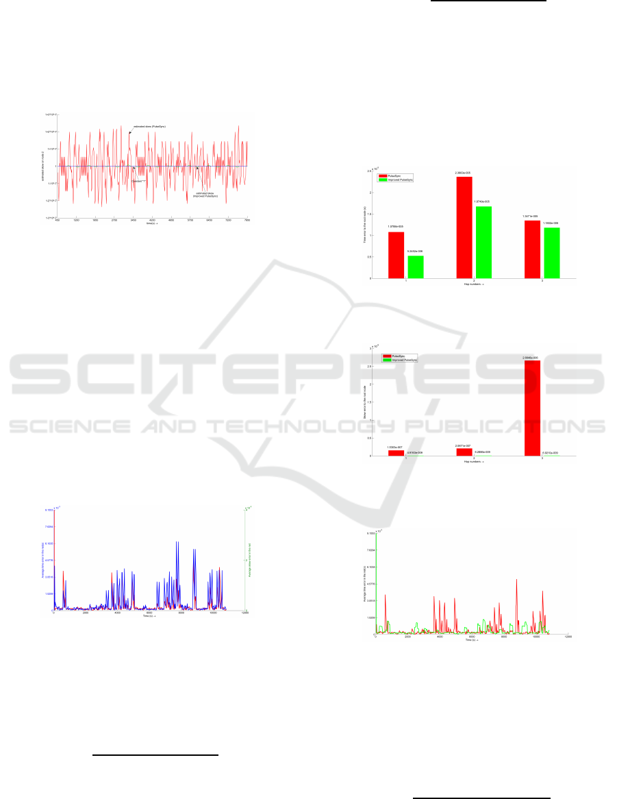
5.5 Simulation
Figure 7: The skew computed on node 2: PulseSync (red)
vs. Improved PulseSync (green).
Finally, the parameters of the Kalman filter are set as
follows:

2ς = 10
−9
γ( j) = 10
−7
(25)
The skews l
2→r
·h
2
|
h
2
=1
that the node 2 computes
with PulseSync and the improved algorithm are plot-
ted on the Figure 7. The blue curve is h
2
(h
2
= 1).
Apparently, the filter is very effective and the stan-
dard deviation of the skew smoothed by the Kalman
Filter only is limited to 2.137 ×10
−9
.
5.6 Results
Figure 8: PulseSync: Average time error in net (red) vs.
average skew error in net (blue).
First, PulseSync is employed to explore the relation-
ships between average time error and average esti-
mated skew error, illustrated in Figure 8. The average
time error in net is defined as follows:
T
ATE
=
∑
i6=r,i∈N


L
i
(t) −L
r
(t)


Num−1
(26)
where Num is the number of nodes in the network. In
this simulation, L
r
(t) is L
1
(t) actually since the node
1 is the root node. The average skew error in net is
defined as follows:
Skew
ATE
=
∑
i6=r,i∈N


ˆ
l
i→r
(t) −1


Num−1
(27)
The global average time error varies with the aver-
age estimated skew error as shown in Figure 8, espe-
cially at time 596, 3636, 7696, 8776 and 10400 sec-
onds. On the other words, the more precise estimated
skew, the less synchronization time error. The im-
proved one has an evident superiority in skew error as
illustrated in Figure 10 and slight better performance
in time error in Figure 9 since that the effect of skew
error has not been amplified through the hops yet.
Figure 9: The time error to the root node with hop numbers:
PulseSync (red) vs. Improved PulseSync (green): the first
three hops.
Figure 10: The skew error to the root node with hop num-
bers: PulseSync (red) vs. Improved PulseSync (green): the
first three hops.
Figure 11: The average time error in net: PulseSync (red)
vs. Improved PulseSync (green).
The comparisons of average time error in net
and neighbor nodes between PulseSync and ours are
shown in Figure 11, Figure 12 respectively. The aver-
age time error between neighbors in net is defined as
follows:
T
ATNE
=
∑
i6=r,i∈N


L
i
(t) −L
i−1
(t)


Num−1
(28)
SENSORNETS 2016 - 5th International Conference on Sensor Networks
102

Figure 12: The average time error between neighbors in net:
PulseSync (red) vs. Improved PulseSync (green).
It is clearly observed that, with the improvedPuls-
eSync, the time error (in Figure 11) does not fluc-
tuate so much and performs well in view of time.
The means of the error during the three hours are
8.8886 ×10
−4
s with PulseSync and 7.6954×10
−4
s
with the improved one respectively. And the stan-
dard deviations of the error during the test periods,
which are used to show how stable the synchro-
nized network are, are 6.5869×10
−4
s (red curve) and
3.0191 ×10
−4
s (green curve).
T
ATNE
shows the synchronization quality among
neighbor nodes. The factor that Kalman filter stabi-
lizes the relative logical clock rate can be observed
in Figure 7 and the effects on the time plotted in
Figure 12 are tangible as well. The mean and stan-
dard deviation of the error during the test periods
are 6.6326 ×10
−4
s and 9.5423 × 10
−6
s with Puls-
eSync, 6.5798×10
−4
s and 4.8146×10
−6
s with the
improved PulseSync.
Figure 13: The skew error to the root node with hop num-
bers: PulseSync (red) vs. Improved PulseSync (green).
Figure 14: The time error to the root node with hop num-
bers: PulseSync (red) vs. Improved PulseSync (green).
Similarly, from the view of hops, the time error
and skew error deviation over multihops decline re-
markably with our algorithm, which can be figured
out from Figure 13, Figure 14. The difference in skew
error is evident at the very start (after 2 hops), also
in time error, the slopes of the zero-crossing linear
fitting are 3.9940×10
−6
and 5.6939×10
−6
respec-
tively. The improved algorithm minimizes the growth
rate of time error with the number of hops. Essen-
tially, these are led by alleviating the clock granular-
ity.
6 CONCLUSIONS
In this work, an improved algorithm based on Puls-
eSync is proposed. Clock granularity impact is alle-
viated by filtering and delivering relativelogical clock
rate, which is beneficial to reducing the deviation of
estimated clock skew through several hops and avails
the accuracy of time synchronization ultimately. The
algorithm is implemented in Contiki OS and simu-
lated in Cooja. Theoretical and experimental analy-
ses show that the novelty on PulseSync works well
in minimizing the multihops error. In the future, we
may revise more sophisticated filter models. Another
direction is to find some better energy efficient syn-
chronization communication mechanism.
ACKNOWLEDGEMENTS
The authors acknowledge the support provided by the
Safety and Emergency Lab of Shanghai Advanced
Research Institute (SARI) for this study. And this
project is supported by ”the Next Generation of In-
formation Technology (IT) for Sensing China” of
Chinese Academy of Sciences (XDA06010800) and
NSFC (61201446).
REFERENCES
Cionca, V., Newe, T., and Dadˆarlat, V. (2008). Tdma pro-
tocol requirements for wireless sensor networks. In
Sensor Technologies and Applications, 2008. SEN-
SORCOMM’08. Second International Conference on,
pages 30–35. IEEE.
Du, J. and Wu, Y. (2013). Distributed clock skew and
offset estimation in wireless sensor networks: Asyn-
chronous algorithm and convergence analysis.
Dunkels, A., Gronvall, B., and Voigt, T. (2004). Contiki-a
lightweight and flexible operating system for tiny net-
worked sensors. In Local Computer Networks, 2004.
29th Annual IEEE International Conference on, pages
455–462. IEEE.
Elson, J., Girod, L., and Estrin, D. (2002). Fine-grained
network time synchronization using reference broad-
Beyond PulseSync: Less Clock Granularity Impact, More Synchronization Accuracy
103

casts. ACM SIGOPS Operating Systems Review,
36(SI):147–163.
Eriksson, J.,
¨
Osterlind, F., Finne, N., Tsiftes, N., Dunkels,
A., Voigt, T., Sauter, R., and Marr´on, P. J. (2009).
Cooja/mspsim: interoperability testing for wireless
sensor networks. In Proceedings of the 2nd Inter-
national Conference on Simulation Tools and Tech-
niques, page 27. ICST (Institute for Computer Sci-
ences, Social-Informatics and Telecommunications
Engineering).
Fan, R. and Lynch, N. (2006). Gradient clock synchroniza-
tion. Distributed Computing, 18(4):255–266.
Ganeriwal, S., Kumar, R., and Srivastava, M. B. (2003).
Timing-sync protocol for sensor networks. In Pro-
ceedings of the 1st international conference on Em-
bedded networked sensor systems, pages 138–149.
ACM.
Lenzen, C., Sommer, P., and Wattenhofer, R. (2009). Op-
timal clock synchronization in networks. In Proceed-
ings of the 7th ACM Conference on Embedded Net-
worked Sensor Systems, pages 225–238. ACM.
Lenzen, C., Sommer, P., and Wattenhofer, R. (2014). Puls-
esync: An efficient and scalable clock synchronization
protocol.
Luo, B. and Wu, Y. (2013). Distributed clock parameters
tracking in wireless sensor network.
Mar´oti, M., Kusy, B., Simon, G., and L´edeczi,
´
A. (2004).
The flooding time synchronization protocol. In
Proceedings of the 2nd international conference on
Embedded networked sensor systems, pages 39–49.
ACM.
Martinez, K., Hart, J. K., Ong, R., Brennan, S., Mielke,
A., Torney, D., Maccabe, A., Maroti, M., Simon, G.,
Ledeczi, A., et al. (2004). Sensor network applica-
tions. IEEE Computer, 37(8):50–56.
Mills, D., Martin, J., Burbank, J., and Kasch, W. (2010).
Network time protocol version 4: Protocol and algo-
rithms specification. IETF RFC5905, June.
Schmid, T., Dutta, P., and Srivastava, M. B. (2010). High-
resolution, low-power time synchronization an oxy-
moron no more. In Proceedings of the 9th ACM/IEEE
International Conference on Information Processing
in Sensor Networks, pages 151–161. ACM.
Sichitiu, M. L. and Veerarittiphan, C. (2003). Simple, ac-
curate time synchronization for wireless sensor net-
works. In Wireless Communications and Network-
ing, 2003. WCNC 2003. 2003 IEEE, volume 2, pages
1266–1273. IEEE.
Sommer, P. and Wattenhofer, R. (2009). Gradient clock syn-
chronization in wireless sensor networks. In Proceed-
ings of the 2009 International Conference on Infor-
mation Processing in Sensor Networks, pages 37–48.
IEEE Computer Society.
Stein, S. R. (1985). 12 frequency and time-their measure-
ment and characterization.
Vig, J. R. (2001). Quartz crystal resonators and oscil-
lators. US Army Communications-Electronics Com-
mand, January.
Wu, Y.-C., Chaudhari, Q., and Serpedin, E. (2011). Clock
synchronization of wireless sensor networks. Signal
Processing Magazine, IEEE, 28(1):124–138.
SENSORNETS 2016 - 5th International Conference on Sensor Networks
104