
Hidden Markov Random Fields and Direct Search Methods for Medical
Image Segmentation
El-Hachemi Guerrout
1
, Samy Ait-Aoudia
1
, Dominique Michelucci
2
and Ramdane Mahiou
1
1
Laboratoire LMCS, Ecole Nationale Sup
´
erieure en Informatique, Oued-Smar, Algiers, Algeria
2
Laboratoire LE2I, Universit
´
e de Bourgogne, Dijon, France
Keywords:
Medical Image Segmentation, Hidden Markov Random Field, Nelder-Mead, Torczon, Kappa Index.
Abstract:
The goal of image segmentation is to simplify the representation of an image to items meaningful and easier to
analyze. Medical image segmentation is one of the fundamental problems in image processing field. It aims to
provide a crucial decision support to physicians. There is no one way to perform the segmentation. There are
several methods based on HMRF. Hidden Markov Random Fields (HMRF) constitute an elegant way to model
the problem of segmentation. This modelling leads to the minimization of an energy function. In this paper
we investigate direct search methods that are Nelder-Mead and Torczon methods to solve this optimization
problem. The quality of segmentation is evaluated on grounds truths images using the Kappa index called also
Dice Coefficient (DC). The results show the supremacy of the methods used compared to others methods.
1 INTRODUCTION
MRI - Magnetic Resonance Imaging, CT - Com-
puted tomography, Radiography, digital mammogra-
phy, and other imaging modalities have indispensable
role in disease diagnosis. However, they produce a
huge number of images for which the manual analy-
sis and interpretation has become a difficult task. The
automatic extraction of meaningful information is one
among the segmentation challenges. In the literature
several approaches have been proposed such as ac-
tive contour models (Kass et al., 1988), edge detec-
tion (Canny, 1986), thresholding (Sahoo et al., 1988),
region growing (Adams and Bischof, 1994), MRF -
Markov Random Fields (Manjunath and Chellappa,
1991), etc.
HMRF - Hidden Markov Random Field, a gener-
alization of Hidden Markov Model (Baum and Petrie,
1966) provides an elegant way to model the seg-
mentation problem. Since the seminal paper of Ge-
man and Geman (1984), Markov Random Fields
(MRF) models for image segmentation have been
investigated intensively (Manjunath and Chellappa,
1991; Panjwani and Healey, 1995; Held et al., 1997;
Hochbaum, 2001; Zhang et al., 2001; Deng and
Clausi, 2004; Kato and Pong, 2006; Yousefi et al.,
2012). The main idea underlying the segmentation
process using HMRF is: the image to segment (called
also the observed image) and the segmented image
(called also the hidden image) are seen like Markov
Random Field. The segmented image is computed
according to the MAP (Maximum A Posteriori) crite-
rion (Wyatt and Noble, 2003). MAP estimation leads
to the minimization of energy function (Szeliski et al.,
2008). This problem is computationally intractable.
In this paper we examine HMRF to model the
segmentation problem and the direct search meth-
ods: Nelder-Mead (Nelder and Mead, 1965) and Tor-
czon (Kolda et al., 2003), as the optimization tech-
niques. In order to evaluate the segmentation quality
we use the Kappa index criterion (Dice, 1945) also
called Dice Coefficient (DC). The Kappa Index cri-
terion gives us how much the segmentation result is
close to the ground truth. The images have been ob-
tained from the Brainweb
1
database (Cocosco et al.,
1997), widely used by the neuroimaging community,
where the ground truth is known.
The achieved results are very satisfactory and
show a superiority of the our proposed methods:
HMRF-Nelder-Mead and HMRF-Torczon, compared
to other methods (Ouadfel and Batouche, 2003;
Yousefi et al., 2012) that are Classical MRF, MRF-
ACO (Ant Colony Optimization) and MRF-ACO-
Gossiping.
This paper is organized as follows. In section 2,
we provide some concepts of Markov Random Field
1
http://www.bic.mni.mcgill.ca/brainweb/
154
Guerrout, E-H., Ait-Aoudia, S., Michelucci, D. and Mahiou, R.
Hidden Markov Random Fields and Direct Search Methods for Medical Image Segmentation.
DOI: 10.5220/0005658501540161
In Proceedings of the 5th International Conference on Pattern Recognition Applications and Methods (ICPRAM 2016), pages 154-161
ISBN: 978-989-758-173-1
Copyright
c
2016 by SCITEPRESS – Science and Technology Publications, Lda. All rights reserved

model. Section 3 is devoted to Hidden Markov Field
model and direct search methods combination to per-
form the segmentation. We give in section 4 some
experimental results. Finally, the section 5 is devoted
to conclusions.
2 HIDDEN MARKOV RANDOM
FIELD MODEL (HMRF)
2.1 Markov Random Field
Let X = {X
1
,X
2
,...,X
M
} be a family of random vari-
ables on the lattice S. Each random variable takes val-
ues in the discrete space Λ = {1,2,...,K}. The fam-
ily X is a random field with configuration set Ω = Λ
M
.
A random field X is said to be an MRF (Markov
Random Field) on S, with respect to a neighborhood
system V (S), if and only if:
∀x ∈ Ω, P[X = x] > 0
∀s ∈ S, ∀x ∈ Ω,P[X
s
= x
s
|X
t
= x
t
,t 6= s] =
P[X
s
= x
s
|X
t
= x
t
,t ∈ V
s
(S)]
(1)
The Hammersley-Clifford theorem (Hammersley &
Clifford, 1971) establishes the equivalence between
Gibbs fields and Markov ones. The Gibbs distribu-
tion is characterized by the following relations:
P[X = x] = Z
−1
e
−U(x)
T
Z =
∑
ξ∈Ω
e
−U(ξ)
T
U(x) =
∑
c∈C
U
c
(x)
(2)
where T is a global control parameter, called tem-
perature, and Z is a normalizing constant, called
the partition function. Calculating Z is prohibitive.
Card(Ω) = 256
512×512
= 2
2097152
for a 512x512 gray
level image. U(x) is the energy function of the Gibbs
field defined as a sum of potentials over all the possi-
ble cliques C.
The local interactions between the neighboring
sites properties (gray levels for example) can be ex-
pressed as a clique potential.
2.2 Standard Markov Random Field
2.2.1 Ising Model
This model was proposed by Ernst Ising for ferro-
magnetism studies in statistical physics. The Ising
model involves discrete variables s (spins), placed
on a sampling grid. Each spin can take two values,
Λ = {−1, 1}. The spins interact in pairs. The first or-
der clique potential is defined by −Bx
s
and the second
order clique potential is defined by:
U
c
2
=
{
s,t
}
(x
s
,x
t
) =
−β if x
s
= x
t
+β if x
s
6=x
t
(3)
U
c
2
=
{
s,t
}
(x
s
,x
t
) = −βx
s
x
t
(4)
The total energy is defined by:
U(x) = −
∑
c
2
={s,t}
βx
s
x
t
−
∑
c
1
={s}
Bx
s
(5)
The coupling constant β, between neighboring sites,
regularize the model and B represents an extern mag-
netic field.
2.2.2 Potts Model
The Potts model is a generalization of the Ising
model. Instead of Λ = {−1,1}, each spin is assigned
an integer value Λ = {1,2,...,K}. In the context of
image segmentation, the integer values are gray levels
or labels. The total energy is defined by:
U(x) = β
∑
c
2
={s,t}
(1 − 2δ(x
s
,x
t
)) (6)
where δ is the Kronecker’s delta:
δ(a,b) =
1 if a = b
0 if a6=b
(7)
When β > 0, the probable configurations correspond
to neighboring sites with same gray level or label.
This induces the constitution of large homogeneous
regions. The size of these regions is guided by the
value of β.
2.3 Hidden Markov Random Field
HMRF is a strong model for image segmentation. The
image to segment is seen as a realization y = {y
s
}
s∈S
of a Markov Random Field Y = {Y
s
}
s∈S
defined on
the lattice S. Each realization y
s
of the random vari-
able Y
s
takes its values in the space of gray levels
Λ
obs
= {0 ...255}. The configuration set of Y is noted
as Ω
obs
. The segmented image is seen as the real-
ization x = {x
s
}
s∈S
of another Markov Random Field
X = {X
s
}
s∈S
, defined on the same lattice S. The real-
ization x
s
of the random variable X
s
takes its values in
the discrete space Λ = {1,2,...,K}. K is the number
of classes or homogeneous regions in the image. The
configuration set of X is noted as Ω.
Figure 1 shows an example of the image to seg-
ment as a realization y of Y and its segmented image
with K = 4 seen as a realization x of X.
In the context of image segmentation, we face a
problem with incomplete data (Dempster et al., 1977).
To every site s ∈ S is associated different information:
Hidden Markov Random Fields and Direct Search Methods for Medical Image Segmentation
155

y: Observed Image x: Hidden Image
Figure 1: Observed and hidden image.
observed information expressed by the random vari-
able Y
s
; missed or hidden information, expressed by
the random variable X
s
. The Random Field X is called
Hidden Markov Random Field.
The segmentation process consists in finding a re-
alization x of X by observing the data of the realiza-
tion y, representing the image to segment.
We seek a labeling ˆx, which is an estimate of the
true labeling x
∗
, according to the MAP (Maximum
A Posteriori) criterion (maximizing the probability
P(X = x|Y = y)).
x
∗
= arg
x∈Ω
max
{
P[X = x|Y = y]
}
(8)
P[X = x|Y = y] =
P[Y = y|X = x]P [X = x]
P[Y = y]
(9)
The first term of the numerator describes the probabil-
ity to observe the image y, knowing the x label. Based
on the assumption of conditional independence, we
get the following formula:
P[Y = y|X = x] =
∏
s∈S
P[Y
s
= y
s
|X
s
= x
s
] (10)
The second term of the numerator describes the exis-
tence of the labeling x. The denominator is constant
and independent of x. We have then:
P[X = x|Y = y] = AP [Y = y|X = x]P [X = x] (11)
where A is a constant, from the equation 2 and 11 we
will have:
P[X = x|Y = y] = Ae
ln(P[Y =y|X=x])−
U(x)
T
(12)
P[X = x|Y = y] = Ae
−Ψ(x,y)
(13)
x
∗
= arg
x∈Ω
min
{
Ψ(x,y)
}
(14)
Maximizing the probability P(X = x |Y = y) is equiv-
alent to minimizing the function Ψ(x,y).
Ψ(x,y) = − ln(P [Y = y|X = x]) +
U(x)
T
(15)
We replace the equation 10 in the equation 15 and we
obtain:
Ψ(x,y) = − ln
∏
s∈S
P[Y
s
= y
s
|X
s
= x
s
]
!
+
U(x)
T
(16)
Ψ(x,y) = −
∑
s∈S
ln(P[Y
s
= y
s
|X
s
= x
s
]) +
U(x)
T
(17)
We assume that the variable [Y
s
= y
s
|X
s
= x
s
] follows a
Gaussian distribution with parameters µ
k
(mean) and
σ
k
(standard deviation). By giving the class label x
s
=
k, we have:
P[Y
s
= y
s
|X
s
= k] =
1
q
2πσ
2
k
e
−(y
s
−µ
k
)
2
2σ
2
k
(18)
The Potts model is often used in image segmentation
to privilege large regions in the image. The energy is
then:
U (x ) = β
∑
c
2
={s,t}
(1 − 2δ (x
s
,x
t
)) (19)
According to equations 17, 18 and 19 we get:
Ψ(x,y) =
∑
s∈S
G
s
+
β
T
∑
c
2
={s,t}
L
s,t
(20)
G
s
= [ln(σ
x
s
) +
(y
s
− µ
x
s
)
2
2σ
2
x
s
]
L
s,t
= (1 − 2δ(x
s
,x
t
))
Optimization techniques to get the estimation ˆx of the
labeling x
∗
are presented in next sections.
3 HMRF AND DIRECT SEARCH
METHODS
Applying the optimization techniques is not obvious.
Thus this section first gives the big picture of our ap-
proach.
Let y = (y
1
,...,y
s
,...,y
M
) be the image to seg-
ment into K classes. Instead of looking for the seg-
mented image x = (x
1
,...,x
s
,...,x
M
) we look for
the vertex µ which contains the means of K classes
µ = (µ
1
,...,µ
j
,...,µ
K
). The segmented image x =
(x
1
,...,x
s
,...,x
M
) is computed by classifying y
s
to
nearest mean µ
j
i.e., if the nearest mean of y
s
is µ
j
then x
s
= j, in the case of tie between two means then
y
s
is classified to the smallest mean.
Let S
j
be the set all the sites s ∈ S in which the
nearest mean to y
s
is µ
j
.
S
j
= {s ∈ S | x
s
= j ⇔ the nearest mean of y
s
is µ
j
}
ICPRAM 2016 - International Conference on Pattern Recognition Applications and Methods
156

Let |S
j
| be the cardinal of S
j
. The standard devia-
tion σ
j
is calculated as follow:
σ
j
=
s
1
| S
j
|
∑
s∈S
j
(y
s
− µ
j
)
2
The image to segment y is known, so if we know
the means µ
j
, then we can compute: its standard devi-
ation σ = (σ
1
,...,σ
j
,...,σ
K
), the segmented image x
and the value of the function Ψ(x,y).
To segment the image, we look for the point
µ = (µ
j
, j = 1 . . . K) where the function Ψ is minimal.
This time, Ψ is seen as a function of µ:
Ψ(µ) =
K
∑
j=1
∑
s∈S
j
G
j,s
+
β
T
∑
c
2
={s,t}
L
s,t
(21)
G
j,s
= [ln(σ
j
) +
(y
s
− µ
j
)
2
2σ
2
j
]
L
s,t
= (1 − 2δ(x
s
,x
t
))
3.1 Direct Search Methods
In this section we explain what we need to apply the
direct search methods for solving our problem defined
above.
The popular Nelder-Mead method or the simplex-
based direct search method was proposed by John
Nelder and Roger Mead (1965). The method starts
with (n + 1) vertices in R
n
that are viewed as the ver-
tices of a simplex. The process of minimizing is based
on the comparison of the function values at (n + 1)
vertices of the simplex, followed by replacing the ver-
tex which has the highest value of the function by
another vertex that can be obtained by operations of
reflection, expansion or contraction relatively to the
center of gravity of the n best vertices of the simplex.
When the substitution conditions are not satisfied, the
method will make the simplex shrink.
Torczon method (1989) (Kolda et al., 2003) comes
to fix gaps of Nelder-Mead like degenerated flat sim-
plices. In the Torczon method, operations are applied
to all vertices of the current simplex, thus by construc-
tion, all simplexes in Torczon method are homothetic
to the first one, and no degeneracy (i.e., ., flat simplex)
can occur.
The stopping criterion in direct search methods is
satisfied when the simplex vertices or their function
values are close.
In our case, we are looking for the best µ ∈
[0...255]
K
which minimizes the function Ψ. For that
we start with a non degenerate simplex with K +1 ver-
tices (coordinates are given in Table 1). When some
vertex is out the bounds (i.e., /∈ [0 . . . 255]
K
), the func-
tion Ψ is set to +∞ (in the practice a very big value).
3.2 HMRF and Nelder-Mead
Combination
We summarize hereafter the Nelder-Mead method
and give examples in two-dimensional space.
HMRF-Nelder-Mead Algorithm.
Repeat.
1. Evaluate
Compute Ψ
i
:= Ψ(V
i
)
Determine the indices h, s, l:
Ψ
h
:= max
i
(Ψ
i
), Ψ
s
:= max
i6=h
(Ψ
i
), Ψ
l
:= min
i
(Ψ
i
)
Compute
¯
V :=
1
K
∑
i6=h
V
i
Example in R
2
(See figure 2)
Figure 2: Center of gravity calculation.
2. Reflect
Compute the reflection vertex V
r
from
V
r
:= 2
¯
V −V
h
Evaluate Ψ
r
:= Ψ(V
r
). If Ψ
l
≤ Ψ
r
< Ψ
s
, replace
V
h
by V
r
and terminate the iteration.
Example in R
2
(See figure 3)
Figure 3: Reflection.
3. Expand
If Ψ
r
< Ψ
l
, compute the expansion vertex V
e
from
V
e
:= 3
¯
V − 2V
h
Evaluate Ψ
e
:= Ψ(V
e
).
If Ψ
e
< Ψ
r
replace V
h
by V
e
and terminate the it-
eration; otherwise (if Ψ
e
≥ Ψ
r
), replace V
h
by V
r
and terminate the iteration.
Example in R
2
(See figure 4)
Hidden Markov Random Fields and Direct Search Methods for Medical Image Segmentation
157
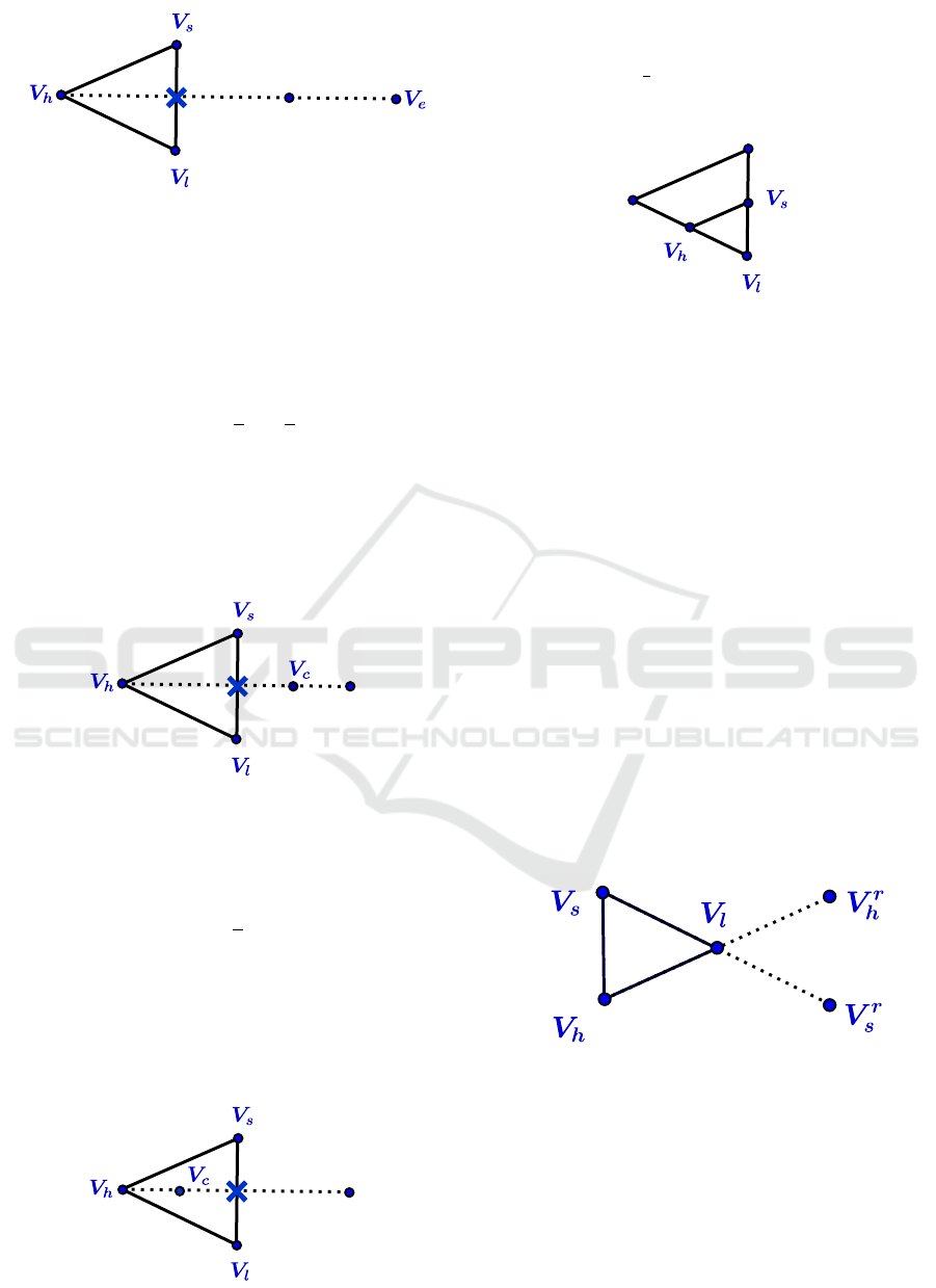
Figure 4: Expansion.
4. Contract
If Ψ
r
≥ Ψ
s
, compute a contraction between
¯
V and
the best of V
h
and V
r
.
(a) Outside contraction
If Ψ
r
< Ψ
h
, compute an outside contraction V
c
from
V
c
:=
3
2
¯
V −
1
2
V
h
Evaluate Ψ
c
:= Ψ(V
c
).
If Ψ
c
< Ψ
r
replace V
h
by V
c
and terminate the
iteration; otherwise ( If Ψ
c
≥ Ψ
r
), go to the
step 5 (shrink).
Example in R
2
(See figure 5)
Figure 5: Outside contraction.
(b) Inside contraction
If Ψ
h
≤ Ψ
r
, compute an inside contraction V
c
from
V
c
:=
1
2
(V
h
+
¯
V )
Evaluate Ψ
c
:= Ψ(V
c
).
If Ψ
c
< Ψ
h
replace V
h
by V
c
and terminate the
iteration; otherwise ( If Ψ
c
≥ Ψ
h
), go to the
step 5 (shrink).
Example in R
2
(See figure 6)
Figure 6: Inside contraction.
5. Shrink
Replace all vertices according to the following
formula V
i
:=
1
2
(V
i
+V
l
)
Example in R
2
(See figure 7)
Figure 7: Shrink.
Until Satisfying a Stopping Criterion.
3.3 HMRF and Torczon Combination
We summarize hereafter the Torczon method and
give examples in two-dimensional space.
HMRF-Torczon Algorithm.
Repeat.
1. Evaluate
Compute Ψ
i
:= Ψ(V
i
)
Determine the indices l from Ψ
l
:= min
i
(Ψ
i
)
2. Reflect
Compute the reflected vertices, V
r
i
:= 2V
l
−V
i
Evaluate Ψ
r
i
:= Ψ(V
r
i
)
If min
i
{Ψ
r
i
} < Ψ
l
go to step 3; otherwise, go to the
step 4
Example in R
2
(See figure 8)
Figure 8: Reflection.
3. Expand
Compute the expanded vertices, V
e
i
= 3V
l
− 2V
i
Evaluate Ψ
e
i
:= Ψ(V
e
i
)
If min
i
{Ψ
e
i
} < min
i
{Ψ
r
i
}, replace all vertices V
i
by
the expanded vertices V
e
i
; otherwise replace all
vertices V
i
by the reflected vertices V
r
i
. In either
case, terminate the iteration.
Example in R
2
(See figure 9)
ICPRAM 2016 - International Conference on Pattern Recognition Applications and Methods
158
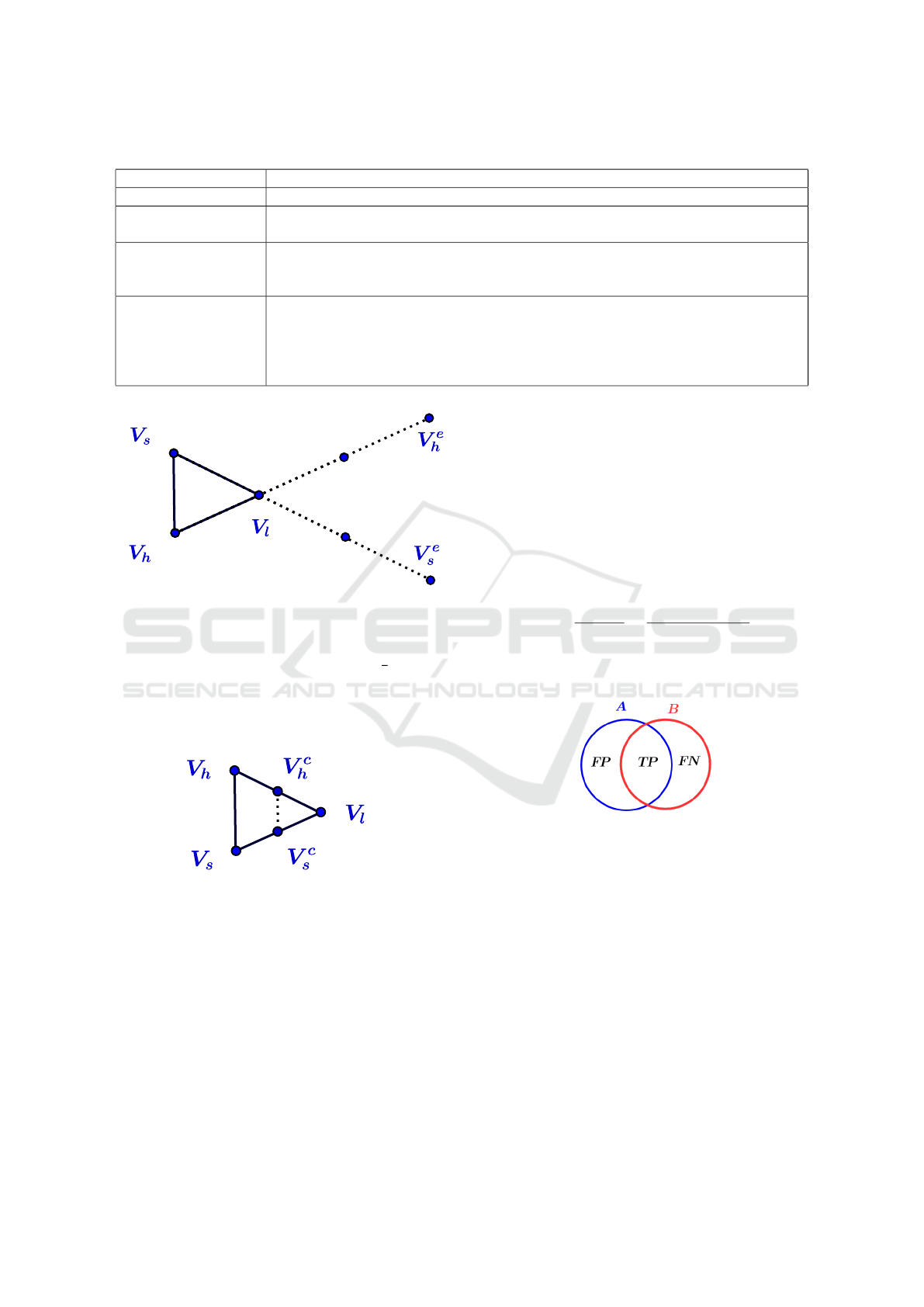
Table 1: Parameters used in our tests.
Method Parameters
Classical MRF T: Temperature=4
MRF-ACO T: Temperature=4, a: Pheromone info. Influence=1, b: Heuristic info. Influence=1,
q: Evaporation rate=0.1, w: Pheromone decay coefficient=0.1
MRF-ACO-
Gossiping
T: Temperature=4, a: Pheromone info. Influence=1, b: Heuristic info. Influence=1,
q: Evaporation rate=0.1, w: Pheromone decay coefficient=0.1, c
1
: Pheromone rein-
forcing coefficient=10, c
2
: Pheromone reinforcing coefficient=100
HMRF-Nelder-Mead
and HMRF-Torczon
T=4, β = 1, vertices of the initial simplex are
V
1
= (196,127,127,127)
V
2
= (127, 63,127,127)
V
3
= (127,127,127,127)
V
4
= (127,127,188,127)
V
5
= (127,127,127,195)
Figure 9: Expansion.
4. Contract
Compute the contracted vertices, V
c
i
=
1
2
(V
i
+V
l
)
Replace all vertices V
i
by the contracted vertices
V
c
i
Example in R
2
(See figure 10)
Figure 10: Contraction.
Until Satisfying a Stopping Criterion.
4 EXPERIMENTAL RESULTS
To assess the two investigated combination meth-
ods referred to as HMRF-Nelder-Mead and HMRF-
Torczon, we made a comparative study with three
segmentation algorithms operating on brain images
that are Classical MRF, MRF-ACO (Ant Colony Op-
timization) and MRF-ACO-Gossiping (Yousefi et al.,
2012). To perform a meaningful comparison, we
use the same medical images with ground truth from
Brainweb database. The comparison is based on the
Kappa Index (or Dice coefficient). We give in table
1 parameters setting for each tested algorithm. The
Dice Coefficient DC (Dice, 1945) or Kappa Index KI
given hereafter allows the visualization of the perfor-
mance of an algorithm. The Dice coefficient between
two classes A and B equals 1 when they are identical
and 0 in the worst case, i.e. no match between A and
B.
KI =
2|A ∩ B|
|A ∪ B|
=
2T P
2T P + FP + FN
(22)
where T P stands for true positive, FP for false posi-
tive and FN for false negative (See figure 11).
Figure 11: TP, FP and FN.
The tables 2 and 3 show respectively the mean
segmentation time and the mean Kappa Index values
of the three classes: GM (Grey Matter), WM (White
Matter), CSF (Cerebro Spinal Fluid) . We have used
the Brainweb database with the parameters: Modal-
ity= T1, Slice thickness = 1mm, Noise = 0% and In-
tensity non-uniformity = 0%. The slices chosen are
used in (Yousefi et al., 2012) which are: 85, 88, 90,
95, 97, 100, 104, 106, 110, 121 and 130.
Figure 12 shows the segmentation result of
HMRF-Nelder-Mead and HMRF-Torczon methods
on a sample of BrainWeb database.
Hidden Markov Random Fields and Direct Search Methods for Medical Image Segmentation
159
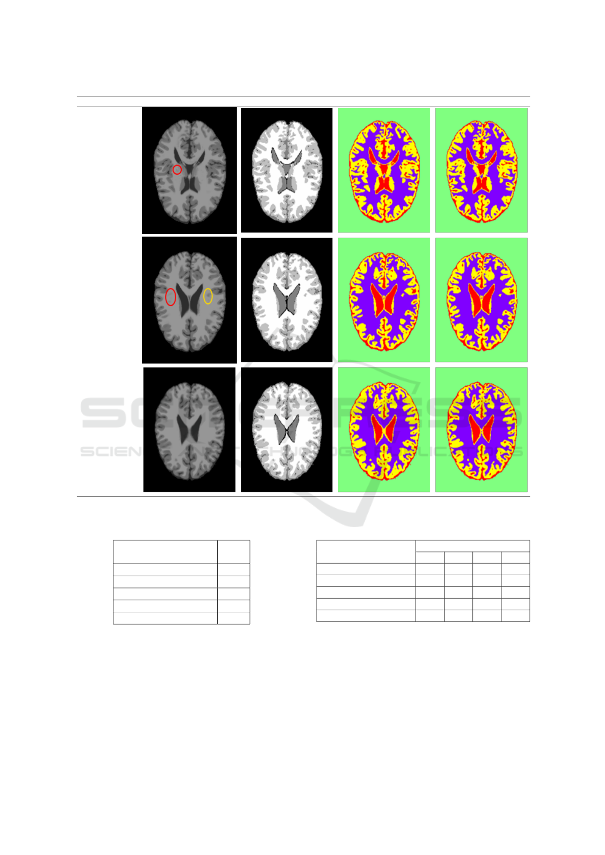
The slice number Original image Ground truth HMRF-Nelder-Mead HMRF-Torczon
88
95
97
Figure 12: Segmentation result of HMRF-Nelder-Mead and HMRF-Torczon methods on a sample of BrainWeb database.
Table 2: The mean segmentation time.
Methods Time
(s)
Classical-MRF 3318
MRF-ACO 418
MRF-ACO-Gossiping 238
HMRF-Nelder-Mead 12.24
HMRF-Torczon 5.55
5 CONCLUSION
In this paper, we have described methods that com-
bine Hidden Markov Random Fields and Direct
Search methods that are Nelder-Mead and Torc-
zon optimisation algorithms to perform segmentation.
Performance evaluation was carried out on sample
Table 3: The mean Kappa Index Values.
Methods
Kappa Index
GM WM CSF Mean
Classical-MRF 0.763 0.723 0.780 0.756
MRF-ACO 0.770 0.729 0.785 0.762
MRF-ACO-Gossiping 0.770 0.729 0.786 0.762
HMRF-Nelder-Mead 0.952 0.975 0.939 0.955
HMRF-Torczon 0.975 0.985 0.956 0.973
medical images from the Brainweb database. From
the tests we have conducted, the combination methods
outperform classical methods. The results are very
promising. Nevertheless, the opinion of specialists
must be considered in the evaluation when no ground
truth is available to have a more synthetic view of the
whole segmentation process.
ICPRAM 2016 - International Conference on Pattern Recognition Applications and Methods
160

REFERENCES
Adams, R. and Bischof, L. (1994). Seeded region grow-
ing. Pattern Analysis and Machine Intelligence, IEEE
Transactions on, 16(6):641–647.
Baum, L. E. and Petrie, T. (1966). Statistical inference for
probabilistic functions of finite state markov chains.
The annals of mathematical statistics, pages 1554–
1563.
Canny, J. (1986). A computational approach to edge detec-
tion. Pattern Analysis and Machine Intelligence, IEEE
Transactions on, (6):679–698.
Cocosco, C. A., Kollokian, V., Kwan, R. K.-S., Pike, G. B.,
and Evans, A. C. (1997). Brainweb: Online interface
to a 3d mri simulated brain database. In NeuroImage.
Citeseer.
Dempster, A. P., Laird, N. M., and Rubin, D. B. (1977).
Maximum likelihood from incomplete data via the em
algorithm. Journal of the royal statistical society. Se-
ries B (methodological), pages 1–38.
Deng, H. and Clausi, D. A. (2004). Unsupervised im-
age segmentation using a simple mrf model with a
new implementation scheme. Pattern recognition,
37(12):2323–2335.
Dice, L. R. (1945). Measures of the amount of ecologic
association between species. Ecology, 26(3):297–302.
Held, K., Kops, E. R., Krause, B. J., Wells III, W. M., Kiki-
nis, R., and Muller-Gartner, H.-W. (1997). Markov
random field segmentation of brain mr images. Medi-
cal Imaging, IEEE Transactions on, 16(6):878–886.
Hochbaum, D. S. (2001). An efficient algorithm for image
segmentation, markov random fields and related prob-
lems. Journal of the ACM (JACM), 48(4):686–701.
Kass, M., Witkin, A., and Terzopoulos, D. (1988). Snakes:
Active contour models. International journal of com-
puter vision, 1(4):321–331.
Kato, Z. and Pong, T.-C. (2006). A markov random field
image segmentation model for color textured images.
Image and Vision Computing, 24(10):1103–1114.
Kolda, T. G., Lewis, R. M., and Torczon, V. (2003). Op-
timization by direct search: New perspectives on
some classical and modern methods. SIAM review,
45(3):385–482.
Manjunath, B. and Chellappa, R. (1991). Unsupervised tex-
ture segmentation using markov random field models.
IEEE Transactions on Pattern Analysis & Machine In-
telligence, (5):478–482.
Nelder, J. A. and Mead, R. (1965). A simplex method
for function minimization. The computer journal,
7(4):308–313.
Ouadfel, S. and Batouche, M. (2003). Ant colony system
with local search for markov random field image seg-
mentation. In Image Processing, 2003. ICIP 2003.
Proceedings. 2003 International Conference on, vol-
ume 1, pages I–133. IEEE.
Panjwani, D. K. and Healey, G. (1995). Markov random
field models for unsupervised segmentation of tex-
tured color images. Pattern Analysis and Machine In-
telligence, IEEE Transactions on, 17(10):939–954.
Sahoo, P. K., Soltani, S., and Wong, A. K. (1988). A survey
of thresholding techniques. Computer vision, graph-
ics, and image processing, 41(2):233–260.
Szeliski, R., Zabih, R., Scharstein, D., Veksler, O.,
Kolmogorov, V., Agarwala, A., Tappen, M., and
Rother, C. (2008). A comparative study of en-
ergy minimization methods for markov random fields
with smoothness-based priors. Pattern Analysis
and Machine Intelligence, IEEE Transactions on,
30(6):1068–1080.
Wyatt, P. P. and Noble, J. A. (2003). Map mrf joint seg-
mentation and registration of medical images. Medi-
cal Image Analysis, 7(4):539–552.
Yousefi, S., Azmi, R., and Zahedi, M. (2012). Brain tis-
sue segmentation in mr images based on a hybrid of
mrf and social algorithms. Medical image analysis,
16(4):840–848.
Zhang, Y., Brady, M., and Smith, S. (2001). Segmenta-
tion of brain mr images through a hidden markov ran-
dom field model and the expectation-maximization al-
gorithm. Medical Imaging, IEEE Transactions on,
20(1):45–57.
Hidden Markov Random Fields and Direct Search Methods for Medical Image Segmentation
161
