Single and Multiple Objective Optimization Models for Opportunistic
Preventive Maintenance
Carlos Henggeler Antunes
1
, Maria João Alves
2
, Joana Dias
2
, Teresa Gomes
1
, Benjamim Cardoso
3
and José Freitas
3
1
Department Electrical and Computer Engineering, University of Coimbra/INESC Coimbra,
Polo 2, 3030-290 Coimbra, Portugal
2
Faculty of Economics, University of Coimbra/INESC Coimbra, Av. Dr. Dias da Silva 165, 3004-512 Coimbra, Portugal
3
Critical Software, Parque Industrial de Taveiro, Lote 49, 3045-504 Coimbra, Portugal
Keywords: Opportunistic Maintenance, Binary Optimization, Multi-objective Models.
Abstract: This paper presents single and multiple objective deterministic optimization models for opportunistic
preventive maintenance of multi-component systems. The single objective model develops an aggregate
cost objective function encompassing costs of replacement, fixed costs associated with maintenance
interventions and costs of component dismounting whenever the replacement of a given component implies
disassembling others. Two multiple objective models are proposed, which enable to explore the trade-offs
between minimizing costs vs. the number of maintenance interventions and minimizing costs vs.
maximizing the remaining lifetime of components at the end of the planning period. Constraints refer to the
requirement of replacing each component before the end of its lifetime and consistency restrictions to allow
opportunistic maintenance and dismounting requirements.
1 INTRODUCTION
Maintenance generally encompasses the care and
servicing by specialized personnel for the purpose of
maintaining equipment and facilities in the required
operating conditions (Ben-Daya et al., 2009). The
primary goal of maintenance is to avoid or mitigate
the consequences of failure of equipment. The
optimization of maintenance operations and
schedule is of utmost importance in industry and
services, in particular in equipment-intensive
industries and utilities (e.g., aviation, energy,
telecommunications, water). Maintenance has a
direct impact on equipment reliability and
availability, and therefore on operational costs. Also,
adequate maintenance and facility management
policies and practices are central in sustaining safety
and eco-efficiency.
Corrective maintenance actions, i.e. those
performed after failure has occurred (run-to-failure),
may result in unwanted system disturbances such as
too frequent shutdowns with the consequent impacts
on costs and quality of service, and even on the
environment.
Preventive maintenance is aimed at preserving
the equipment operating conditions and preventing
their (otherwise costly) failure, involving partial or
complete overhauls to preserve and restore
equipment reliability. It provides for systematic
inspection, detection, and correction of emerging
failures before they happen or develop into major
faults. It may include tests, measurements,
adjustments and component replacement to prevent
faults from occurring. In general, preventive
maintenance is regularly or condition-based
performed on an equipment, or worn components,
often still working, to lessen the likelihood of
failing. Therefore, production loss, downtime, and
safety and environmental hazards are minimized.
Preventive maintenance is generally scheduled
based on a time or usage activation signal. An air-
conditioner is a typical example of an asset for
which a time-based preventive maintenance
schedule is performed: e.g., it is checked every year,
before the hot season. An example of an asset with a
usage-based preventive maintenance schedule is a
motor vehicle that should be scheduled for service
every 20,000 km. Applications that are generally
mentioned as suitable for preventive maintenance
Antunes, C., Alves, M., Dias, J., Gomes, T., Cardoso, B. and Freitas, J.
Single and Multiple Objective Optimization Models for Opportunistic Preventive Maintenance.
DOI: 10.5220/0005661601070114
In Proceedings of 5th the International Conference on Operations Research and Enterprise Systems (ICORES 2016), pages 107-114
ISBN: 978-989-758-171-7
Copyright
c
 2016 by SCITEPRESS – Science and Technology Publications, Lda. All rights reserved
107

include those that have a critical operational
function, failure modes that can be prevented with
regular maintenance, or a likelihood of failure that
increases with time or usage.
Since the maintenance schedule should be
planned, preventive maintenance is more complex to
coordinate than corrective maintenance. In this
scope, maintenance should be mainly seen as
investment in reliability and availability rather than a
cost-inducing activity. Therefore, optimization
approaches are required, aimed at encompassing the
essential features of real-world maintenance
problems in different settings, i.e. taking into
account the specificities of each industry and their
equipment usage, in order to generate optimal
recommendations to planners and decision makers.
In this setting, opportunistic maintenance models
are well suited to several real-world problems, thus
accommodating flexible strategies for planning
maintenance activities (Dekker et al., 1997).
Opportunistic models, i.e. preventive maintenance
activities at an opportunity, entail deciding whether
additional maintenance activities beyond the ones
that are strictly required should be performed at a
(possibly already planned) maintenance occasion.
I.e., if the system is already under maintenance
(either working or in a shutdown mode),
components may be replaced or maintained at no
additional fixed cost for intervention. Opportunistic
maintenance optimization using deterministic
models has been considered by Epstein and
Wilamowsky (1985), Dickman et al. (1990), Nilsson
et al. (2009) and Almgren et al. (2012), among
others. Stochastic opportunistic replacement models
have also been studied by several authors including
the recent work by Patriksson et al. (2015).
In this paper single and multiple objective
deterministic mathematical models are developed to
provide decision support in the scheduling of
opportunistic maintenance activities. Decisions to be
made involve component replacement and
component dismounting whenever the replacement
of a given component implies disassembling others.
The single objective function aggregates these
different costs to determine the optimal solution.
The single objective model has been developed from
the basic opportunistic replacement model by
Almgren et al. (2012) by including component
dismounting actions.
Two models with multiple objective functions
are then proposed, which enable to explore the trade-
offs between minimizing replacement and
dismounting costs vs. minimizing the number of
maintenance interventions and minimizing total
costs vs. maximizing the remaining lifetime of
components at the end of the planning period. For
multi-objective models the nondominated (Pareto
optimal) set is computed. A feasible solution is
nondominated if no other feasible solution exists that
simultaneously improves all objective function
values, i.e. improving an objective function implies
worsening the value of at least another objective
function value. In the present work the whole
nondominated set has been obtained using a
procedure based on reference points co-developed
by one of the authors (Alves and Clímaco, 2000).
In section 2 a single objective model for
optimizing opportunistic maintenance is presented,
in which an overall cost objective function is
considered. Multi-objective models for decision
support in opportunistic maintenance are presented
in section 3. Conclusions are drawn and further
research is outlined in section 4.
2 A SINGLE OBJECTIVE MODEL
FOR OPTIMIZING
OPPORTUNISTIC
MAINTENANCE
In this section a single objective mathematical model
devoted to optimize the maintenance scheduling of a
multi-component system is presented. The
components must be replaced before they reach the
end of their lifetime; this is estimated so that the
probability of a component failure within its lifetime
is low enough for its intended use and is usually
provided by the equipment manufacturer. Hence, a
deterministic model is considered under this
assumption.
Considering a set of components and a finite
planning horizon discretized in time intervals, the
model aims at determining the dismounting and
replacement schedule of the components during the
planning horizon in order to minimize the total cost.
A component that is replaced must be firstly
dismounted. In addition, the replacement of a given
component may imply dismounting others in which
the component is embedded, regardless of whether
those components require or not maintenance at that
time interval.
Opportunistic maintenance is mainly justified
when there is a significant fixed cost associated with
a maintenance intervention, which is independent of
the components that are replaced. The proposed
model considers an overall cost objective function
including terms related to fixed (opportunity) costs
ICORES 2016 - 5th International Conference on Operations Research and Enterprise Systems
108

for interventions and costs for component
replacement and dismounting.
Constraints refer to:
- the requirement of replacing each component
before the end of its lifetime, including considering
that at the beginning of the planning period some
components may be already worn out (i.e. having
some time of use);
- enforcing the consideration of the fixed cost for
intervention if at least one component is replaced at
a given time interval (to induce maintenance
opportunities at no additional fixed cost);
- requirement of dismounting a component if it
contains another component that is replaced.
2.1 Single Objective Model
The model inputs are:
- A set of N components, which are the target of
the replacement/maintenance actions.
- A set of T time intervals, which result from the
discretization of the finite planning horizon.
- A maximum replacement interval L
i
for each
component i ∈{1,…,N} corresponding to its
estimated lifetime (this maximum replacement
interval can also derive from a policy decision, a
safety regulation associated with the component’s
technical life, or a contractual requirement).
L
0i
is the maximum replacement interval for each
component i for the first time in the planning period
T, thus taking into account its time of use before
t =0.
- The replacement cost c
it
of component i
∈{1,…,N} at time t ∈{1,…,T}.
- The fixed cost associated with a maintenance
intervention (opportunity cost) d
t
≥ 0 at time t
=1,…,T, which is independent of the number of
components replaced.
- The replacement of a component implies that it
should be firstly dismounted. The dismounting cost
of component i at time t is a
it
.
- If component i is embedded into other
component(s) then it may happen that in order to
dismount component i it is necessary to dismount
other component(s) as well. Let M(i) be the set of
components j that should be dismounted when
component i is dismounted.
Decision variables:
x
it
= 1, if component i ∈{1,…,N} is replaced at
time t ∈{1,…,T}; 0, otherwise.
y
it
= 1, if component i ∈{1,…,N} is dismounted
at time t ∈{1,…,T}; 0, otherwise.
w
t
= 1, if at least one replacement operation
occurs at time t ∈{1,…,T}; 0, otherwise.
The single objective model is:
Model S1
∑∑
==
⎟
⎟
⎠
⎞
⎜
⎜
⎝
⎛
++
T
t
N
i
ttitititit
wdyaxc
11
)(min
(1)
subject to:
∑
=
=≥
i
L
t
it
Nix
0
1
,...,1 ,1
(2)
∑
+
+=
=−=≥
i
Lk
kt
iit
NiLTkx
1
,...,1 ;,...,1 ,1
(3)
NiTtwyx
titit
,...,1 ;,...,1 , ==≤≤
(4)
M(i)jTtyy
jtit
∈=≤ ;,...,1 ,
,∀i:M(i)≠∅
(5)
NiTtwyx
titit
,...,1 ;,...,1 }1,0{,, ==∈
(6)
The objective function (1) minimizes the total
cost considering the component replacement,
component dismounting and fixed costs for
interventions. Constraints (2) ensure that each
component is replaced within its maximum
replacement interval for the first time and (3) ensure
the replacement of each component before the end
of its lifetime for the rest of the planning period.
Constraints (4) ensure that a component is
dismounted before it is replaced and an intervention
operation occurs at that time interval. Constraints (5)
impose that each component j in which i is
embedded is also dismounted if i is dismounted.
The model (1)-(6) can be simplified to have
fewer variables and constraints, and thus minimize
the computational effort.
Let
∪
N
i
iMM
1
)(
=
=
.
The y
jt
variables will be defined only for j ∈ M.
Therefore, consider the following definitions:
x
it
= 1, if component i ∈{1,…,N} is dismounted
and replaced at time t ∈{1,…,T}; 0, otherwise.
y
jt
= 1, if component j ∈ M is dismounted at time
t ∈{1,…,T}; 0, otherwise.
w
t
keeps the same definition as above.
The simplified model is:
Model S2
∑
∑∑ ∑∑
=
== ∈∉
+
⎟
⎟
⎠
⎞
⎜
⎜
⎝
⎛
++
T
t
tt
T
t
N
iMj
jtjt
Mi
itititit
wd
yaxaxc
1
11
min
(7)
subject to:
∑
=
=≥
i
L
t
it
Nix
0
1
,...,1 ,1
(8)
Single and Multiple Objective Optimization Models for Opportunistic Preventive Maintenance
109

∑
+
+=
=−=≥
i
Lk
kt
iit
NiLTkx
1
,...,1 ;,...,1 ,1
(9)
NiTtwx
tit
,...,1 ;,...,1 , ==≤
(10)
MjTtyx
jtjt
∈=≤ ;,...,1
(11)
M
(i)jTtyx
jtit
∈=≤ ;,...,1 ,
,∀i:M(i)≠∅
(12)
, , {0,1} 1,..., ; 1,..., ;
it t jt
x
wy t T i Nj M∈= = ∈
(13)
The model (7)-(13) has the same number of
variables and constraints as the model (1)-(6) only if
|M|=N. Otherwise it has fewer variables and
constraints. Constraints (10) and (11) correspond to
constraints (4) in Model S1 and constraints (12)
correspond to (5). Remind that x
it
= 1 means that
component i is dismounted and replaced at time t, so
variables y
jt
can be directly related to x
it
for which y
it
have not been defined (i.e., for i ∉ M). The fact that
y variables are not defined for all components leads
to a different formulation of the cost function (7),
associating the dismounting cost with y
jt
for
components j∈M and with x
it
for i ∉ M.
As only superfluous variables (and related
constraints) are eliminated from Model S1 to Model
S2, the two models are equivalent.
2.2 Illustrative Example
Model S2, (7)-(13), has been instantiated with the
following data for illustrative purposes: N=5
components and T=50 time intervals.
Table 1 displays the lifetime (L
0i
and L
i
), costs
for each component (c
it
and a
it
) and dismounting
requirements (M(i)).
Experiments have been carried out with fixed
costs for interventions d
t
= 10, 100, 1000, for all t.
Table 1: Lifetime, costs for each component (costs are the
same for all time intervals) and dismounting requirements.
Component 1 2 3 4 5
L
0i
2 5 11 4 15
L
i
7 10 16 9 20
c
i
t
80 185 160 125 150
a
i
t
20 45 40 30 35
M(i)
∅ ∅
1 2, 5
∅
These instances have 450 binary variables and
743 constraints. The equivalent Model S1 would
lead to instances with 550 binary variables and 843
constraints.
Tables 2-4 present optimal solutions for d
t
= 10,
100, 1000, respectively. “x” denotes component
replacement and “o” denotes dismounting without
replacement. These solutions were obtained using
our software for MultiObjective Mixed-Integer
Linear Programming (MOMILP) problems (see
section 3), which uses the non-commercial lpsolve55
software (http://lpsolve.sourceforge.net/5.5/) to
solve the integer single-objective problems. The
computation times for obtaining the optimal
solutions to the problems with d
t
= 10, 100 and
1000, in a computer with Intel Core i7-2600K
CPU@3.4GHz and 8 GB RAM, were 0.05, 2.65 and
0.08 seconds, respectively.
Table 2: Optimal solution for d
t
= 10.
Component →
Interval↓
1 2 3 4 5
2 x
4 x x o
9 x x
13 x x x
16 x o x o
23 x x x
24 o x o
30 x
33 x x x
37 x x
42 x x o
44 x
The total cost of the optimal solution for d
t
= 10
(Table 2) is 4100, 3980 for dismounting and
replacing plus 120 for intervention fixed cost, with
12 maintenance interventions being made.
Table 3: Optimal solution for d
t
= 100.
Component →
Interval↓
1 2 3 4 5
2 x
4 x x x o
10 x x
13 x x x
17 x
22 x x o
24 x x
31 x x x x
38 x o x x o
41 x
44 x o x o
The total cost of the optimal solution for d
t
= 100
(Table 3) is 5180, 4080 for dismounting and
replacing plus 1100 for intervention fixed cost, with
11 maintenance interventions.
The total cost of the optimal solution for d
t
=
1000 (Table 4) is 11690, 4690 for dismounting and
replacing plus 7000 for intervention fixed cost, with
7 maintenance interventions.
ICORES 2016 - 5th International Conference on Operations Research and Enterprise Systems
110

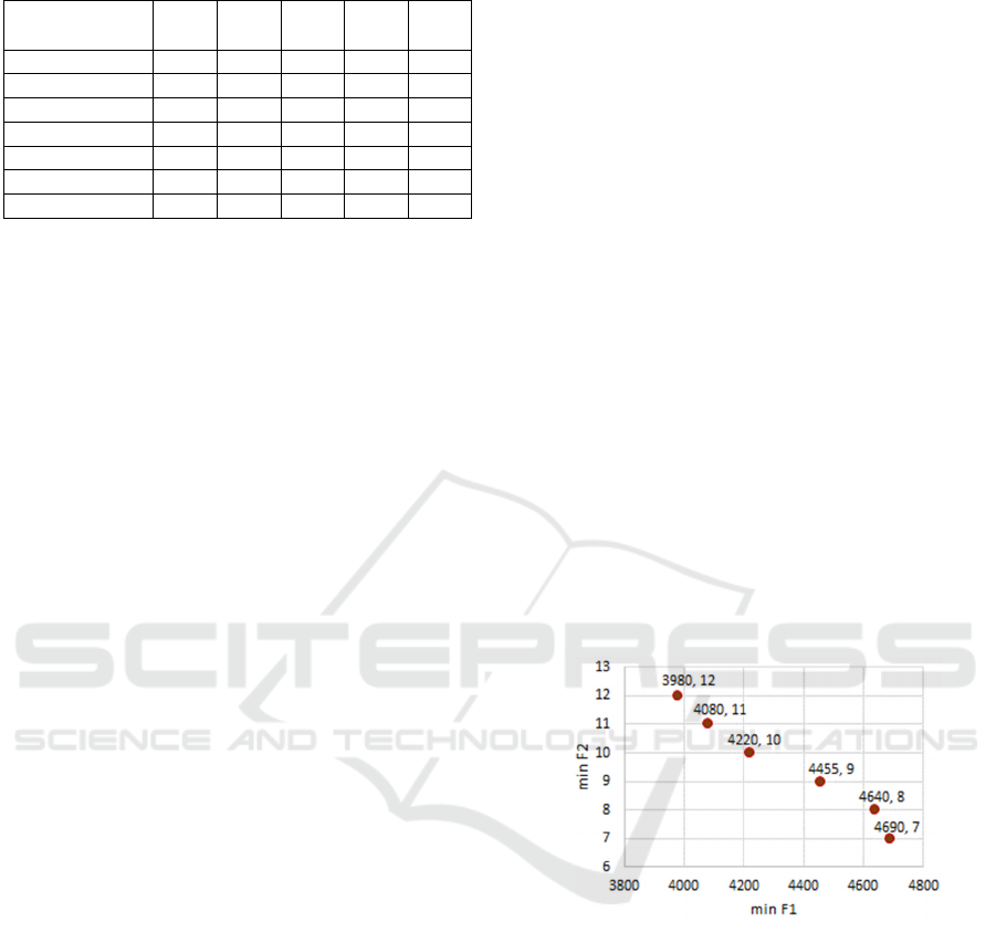
Table 4: Optimal solution for d
t
= 1000.
Component →
Interval↓
1 2 3 4 5
2 x x x o
9 x x x x x
16 x x x o
23 x x x x x
30 x x x o
37 x x x x x
44 x x x o
The total cost of the optimal solution for d
t
=
1000 (Table 4) is 11690, 4690 for dismounting and
replacing plus 7000 for intervention fixed cost, with
7 maintenance interventions.
We can observe from these solutions that there is
frequent disassembling of component 5 due to the
frequent replacement of component 4, which has a
short lifetime. Although the replacement of
component 3 requires disassembling the component
1, it is not necessary to disassemble component 1
without its replacement in any solution because this
component has a short lifetime and low replacement
cost. Finally, it should be mentioned that solutions
for d
t
=10 and d
t
=100 (Tables 2-3) have several
optimal alternative solutions, i.e. different
combinations of component replacement and
disassembling in the planning period leading to the
same optimal objective function value.
This model requires the specification of fixed
costs for interventions d
t
, which in some cases may
be difficult to estimate. In order to better explore
compromises between cost (of replacement and
dismounting) and number of maintenance
interventions, a bi-objective model is proposed
below.
3 MULTIPLE OBJECTIVE
MODELS FOR DECISION AID
IN OPPORTUNISTIC
MAINTENANCE
In this section bi-objective models are proposed,
which enable to explore the trade-offs between
minimizing replacement and dismounting costs vs.
the number of maintenance interventions (Model
M1) and minimizing total costs vs. maximizing the
remaining lifetime of components at the end of the
planning period (Model M2). The results of the
illustrative examples were obtained using the
interactive MOMILP software co-developed by one
of the authors in Delphi for Windows (Alves and
Clímaco, 2004), which includes a reference point-
based procedure that is able to compute the whole
nondominated front for bi-objective problems.
3.1 Minimizing Costs Vs. Number of
Maintenance Interventions
The first objective function (14) of Model M1
minimizes the replacement and dismounting cost
while the second objective function (15) aims at
minimizing the number of maintenance
interventions.
Model M1
∑∑ ∑∑
== ∈∉
⎟
⎟
⎠
⎞
⎜
⎜
⎝
⎛
++=
T
t
N
iMj
jtjt
Mi
itititit
yaxaxcF
11
1
min
(14)
∑
=
=
T
t
t
wF
1
2
min
(15)
subject to:
(8) – (13)
Example:
Model M1 has been instantiated with the same
data as the single-objective model. The resulting
problem has 7 nondominated solutions, which are
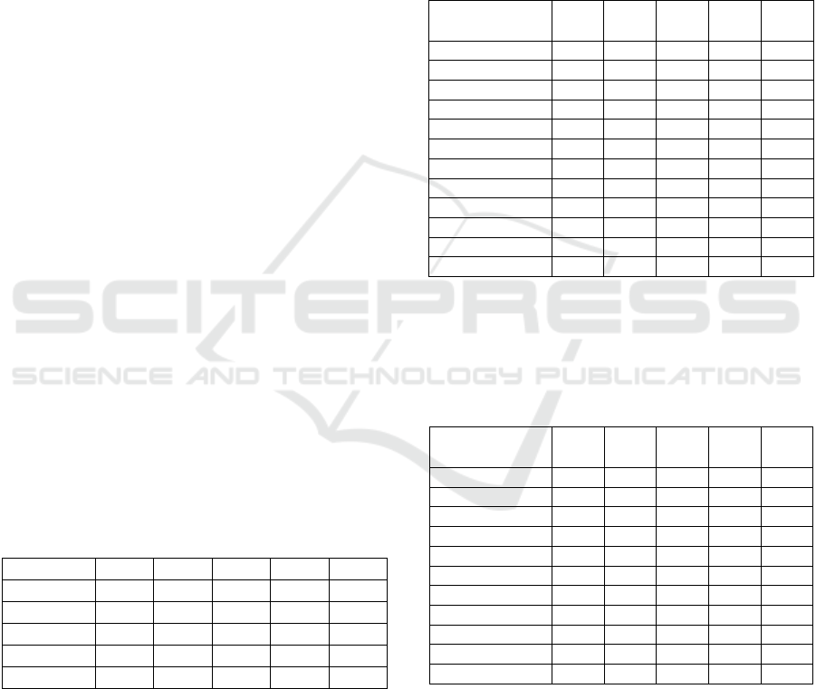
depicted in Figure 1.
Figure 1: Nondominated front: replacement and
dismounting cost vs. number of interventions (Model M1).
The nondominated solution that minimizes cost,
(F
1
, F
2
) = (3980, 12), is an alternative optimal
solution to the single objective model with the
smaller value of d
t
, i.e. d
t
=10. The nondominated
solution that minimizes the number of maintenance
interventions, (F
1
, F
2
) = (4690, 7), is the optimal
solution to the single objective model with d
t
=1000.
The solution where (F
1
, F
2
) = (4080, 11) is an
alternative optimal solution for the single objective
model with d
t
=100. In addition to these solutions,
there are other intermediate nondominated solutions
with 8, 9 and 10 interventions. Note that several
alternative configurations (decision variable values)
Single and Multiple Objective Optimization Models for Opportunistic Preventive Maintenance
111

can be found for the same nondominated objective
point. This happens, in particular, for the solutions
that consider a large number of maintenance
interventions. However, the nondominated points
(objective function values) are only those shown in
Figure 1.
3.2 Minimizing Total Cost Vs.
Maximizing the Remaining
Lifetime of Components at the End
of the Planning Period
In addition to the minimization of maintenance
costs, the maximization of the value of the assets at
the end of the planning period may also be an
objective the decision maker wants to accomplish,
namely if the planning period should be extended
due to any circumstance. The real value of a
component depends on its remaining lifetime. The
next model (Model M2) considers again the overall
cost (replacement and dismounting plus the
intervention fixed cost) for the first objective
function. Thus, its formalization (16) is the same as
the objective function (7) of the single objective
model. The second objective function aims at
maximizing the remaining lifetime of the
components, as a proxy for maximizing the value of
the assets at the end of the planning period. As the
decision maker may want to assign different levels
of importance to each component, a weighted sum of
the remaining lifetime of the components is
considered. This objective function is formalized in
(17), where α
i
denotes the weight assigned to each
component i.
If the component i is replaced at the last time
interval of the planning period, t=T, then its
remaining lifetime is L
i
; if the replacement is at
t =T-1, then its remaining lifetime is L
i
– 1, and so
on; thus the remaining lifetime of the component at
the end of the planning period can be given by
∑
+−=
T
LTt
itit
i
xv
1
with
kLv
iit
−=
for
kTt −=
, provided
the model ensures that the component is replaced
only once from the time
i
LT −
to T. Accordingly,
the replacement constraints of each component for
the last period, i.e. constraints (9) for
i
LTk −=
,
are changed to be of type “=” instead of “≥”. These
are constraints (19) in Model M2; the other
constraints of (9) are replaced by (18) in this model.
Model M2
∑
∑∑ ∑∑
=
== ∈∉
+
⎟
⎟
⎠
⎞
⎜
⎜
⎝
⎛
++=
T
t
tt
T
t
N
iMj
jtjt
Mi
itititit
wd
yaxaxcF
1
11
1
min
(16)
∑∑
=+−=
⎟
⎟
⎠
⎞
⎜
⎜
⎝
⎛
α=
N
i
T
LTt
ititi
i
xvF
11
2
max
(17)
subject to:
(8), (10) – (13)
∑
+
+=
=−−=≥
i
Lk
kt
iit
NiLTkx
1
,...,1 ;1,...,1 ,1
(18)
∑
+−=
==
T
LTt
it
i
Nix
1
,...,1 ,1
(19)
Examples:
Model M2 has been instantiated with the same
data as the previous models using d
t
=100.
Two experiments were performed. The first one
considered α
i
=1 for all i. In the second experiment
higher weight was given to components with smaller
lifetime: α
i
=1/L
i
. The weights were then normalized
so that
N
N
i
i
=α
∑
=1
. The normalization enables a
better comparison between the two experiments as
the weights have equal sum.
In the first experiment 23 nondominated
solutions were obtained, which are depicted in figure
2. The overall cost ranges from 5180 to 6230. The
solution with minimum cost (solution A in Figure 2,
shown in Table 5) presents a sum of remaining
lifetime at the end of the planning period of 14.
Table 5 also shows the remaining lifetime of each
component. This solution is an alternative optimal
solution to the single objective Model S2 with
d
t
=100. However, the optimal solution of Model S2
presented in Table 3 has a sum of remaining lifetime
of only 9. Solution A is also an alternative to the
nondominated solution that minimizes cost in the bi-
objective Model M1 (cost vs. number of
maintenance interventions). Likewise, the number of
maintenance interventions is equal to 11. However,
the sum of remaining lifetime is 12 in the solution
obtained for Model M1, which is worse than the
corresponding value in solution A for Model M2.
Hence, the nondominated solution that minimizes
cost obtained for Model M2 may be more interesting
than the solutions that minimize cost for the single
objective Model S2 and the multiobjective Model
M1: all these solutions have the same cost and
number of maintenance interventions but solution A
ICORES 2016 - 5th International Conference on Operations Research and Enterprise Systems
112

presents a larger overall remaining lifetime at the
end of the planning period.
The nondominated solution that maximizes the
sum of remaining lifetime (solution B in Figure 2,
shown in Table 6) has a value of 62 for this
objective and a total cost of 6230. This solution
proposes the replacement of all components at the
last time interval of the planning period, i.e. t =
T =50, so it ensures the maximum remaining lifetime
for all components.
Figure 2: Nondominated front: overall cost vs. sum of
remaining lifetime at the end of the planning period
(Model M2 – experiment 1).
Table 5: Solution A that minimizes cost in Model M2.
Component →
Interval↓
1 2 3 4 5
1 x o x o
5 x
8 x o x x o
15 x x x x
22 x x
24 x x o
29 x
33 x x x
36 x x
42 x x x o
49 x
remaining lifetime 6 2 2 1 3
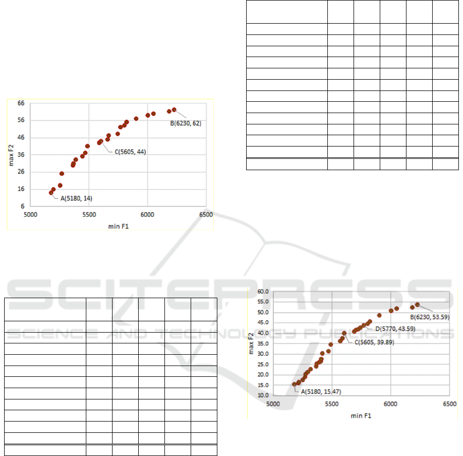
In the second experiment, considering a
weighted-sum for the remaining lifetime objective
function, 31 nondominated solutions were obtained,
which are depicted in Figure 3. The extreme
solutions (A and B), which optimize individually
each objective function, are similar in both
experiments. The problem solved in the second
experiment has more nondominated solutions than
the one solved in the first experiment (with equal
weights) and some solutions are common, but not all
solutions of the first problem belong to the
nondominated set of the second problem.
Table 6: Solution B that maximizes the sum of remaining
life in Model M2.
Component →
Interval↓
1 2 3 4 5
2 x x x o
9 x x
11 x x x
13 x
20 x x x x o
27 x o x o
30 x x
34 x o x x o
40 x x
41 o x o
43 x
50 x x x x x
remaining lifetime 7 10 16 9 20
An intermediate solution obtained in these
experiments with Model M2 can also be analyzed,
e.g. solution C (Figures 2 and 3), common to both
experiments. The solution configuration is presented
in Table 7. It requires 12 maintenance interventions.
The total cost is 5605 and the sum of remaining
lifetime is 44 (the weighted sum of remaining
lifetime is 39.89 – value of F
2
in the second
experiment).
Figure 3: Nondominated front: overall cost vs. weighted
sum of remaining life at the end of the planning period
(Model M2 – experiment 2).
We can observe in Table 7 that four of the five
components (1, 2, 4 and 5) are replaced near the end
of the planning period, i.e., at t=49, so their
remaining lifetime is near the respective maximum
(L
i
−1). However, the last replacement of component
3 is at t=36, so its remaining lifetime at the end of
the planning period is only 2. Therefore, although
intermediate solutions exist displaying a good trade-
off between cost and (weighted) sum of remaining
lifetime at the end of the planning period, the
individual remaining lifetimes may not be balanced
among the various components. Solution D in Figure
Single and Multiple Objective Optimization Models for Opportunistic Preventive Maintenance
113

3 also needs 12 maintenance interventions. The last
replacement of each component occurs at t=48,
leading to a remaining lifetime of 5, 8, 14, 7 and 18,
respectively for components 1 to 5. The minimum
remaining lifetime is 5, thus the remaining lifetimes
are more balanced than in solution C. However,
solution D presents a higher cost than C (5770 vs.
5605).
Table 7: Solution C to Model M2.
Component →
Interval↓
1 2 3 4 5
1 x
4 x x o
8 x x
13 x x x
15 x
22 x x x x o
29 x x
31 x x o
36 x x
40 x x o
43 x
49 x x x x
remaining lifetime 6 9 2 8 19
4 CONCLUSIONS
Single and multiple objective deterministic
optimization models have been presented to support
opportunistic preventive maintenance decisions
regarding a set of components, which are the target
of the replacement/maintenance actions, over a finite
planning horizon. The single objective model
considers the minimization of an overall cost
objective function including fixed costs for
interventions and costs for component replacement
and dismounting whenever the replacement of a
given component implies disassembling others. The
multi-objective models enable to explore the trade-
offs between minimizing replacement and
dismounting costs vs. the number of maintenance
interventions and minimizing total costs vs.
maximizing the remaining lifetime of components at
the end of the planning period. Illustrative examples
have been presented using software developed by
some of the authors for general multiobjective
mixed-integer programming problems to exploit the
practical insights offered by the models.
Further research will involve developing
adequate sensitivity analysis techniques to take into
account the uncertainty associated with the model
coefficients to obtain robust solutions, i.e.
recommendations that are relatively immune to
changes of coefficients within plausible ranges.
Moreover, the models will be exploited in real-world
settings taking into account the particularities raised
by specific situations as well as scalability issues to
tackle large-scale problems in systems with
hundreds of components.
ACKNOWLEDGEMENTS
The authors acknowledge the support of iAsset
Project, ref. 38635/2014, financed by POFC, and
FCT project grants UID/MULTI/00308/2013 and
MITP-TB/CS/0026/2013.
REFERENCES
Alves, M. J., Clímaco, J., 2000. An interactive reference
point approach for multiobjective mixed-integer
programming using branch-and-bound. European
Journal of Operational Research, 124 (3), 478-494.
Alves, M. J., Clímaco, J., 2004. A note on a decision
support system for multiobjective integer and mixed-
integer programming problems. European Journal of
Operational Research, 155(1), 258-265.
Almgren, T., Andréasson, N., Patriksson, M., Strömberg,
A. B., Wojciechowski, A., & Önnheim, M., 2012. The
opportunistic replacement problem: theoretical
analyses and numerical tests. Mathematical Methods
of Operations Research, 76(3), 289-319.
Ben-Daya, M., Duffuaa, S.O., Raouf, A., Knezevic, J.,
Ait-Kadi, D. (Eds.), 2009. Handbook of Maintenance
Management and Engineering, Springer.
Dekker, R., Wildeman, R.E., van der Duyn-Schouten,
F.A., 1997. A review of multi-component maintenance
models with economic dependence, Mathematical
Methods of Operations Research, 45, 411-435.
Dickman, B., Wilamowsky, Y., Epstein, S., 1990.
Modeling deterministic opportunistic replacement as
an integer programming problem. American Journal of
Mathematical and Management Sciences, 10(3-4),
323-339.
Epstein, S., Wilamowsky, Y., 1985. Opportunistic
replacement in a deterministic environment.
Computers & Operations Research, 12(3), 311-322.
Nilsson, J., Wojciechowski, A., Strömberg, A. B.,
Patriksson, M., Bertling, L., 2009. An opportunistic
maintenance optimization model for shaft seals in
feed-water pump systems in nuclear power plants. In
2009 IEEE Bucharest Power Tech Conference.
Patriksson, M., Strömberg, A. B., Wojciechowski, A.,
2015. The stochastic opportunistic replacement
problem, part I: models incorporating individual
component lives. Annals of Operations Research,
224(1), 25-50.
ICORES 2016 - 5th International Conference on Operations Research and Enterprise Systems
114