Techniques to Control Robot Action Consisting of Multiple Segmented

Motions using Recurrent Neural Network with Butterﬂy Structure

Wataru Torii, Shinpei Fujimoto, Masahiro Furukawa, Hideyuki Ando and Taro Maeda

Information Science, Graduate School of Osaka University, Yamadaoka 2-1, 560-0871, Suita-shi, Osaka, Japan

Keywords:

Robot Manipulation, RNN, FFT Butterﬂy, Associative Memory, ”Tsumori”.

Abstract:

In the ﬁeld of robot control, there have been several studies on humanoid robots operating in remote areas. We

propose a methodology to control a robot using input from an operator with fewer degrees of freedom than

the robot. This method is based on the concept that time-continuous actions can be segmented because human

intentions are discrete in the time domain. Additionally, machine learning is used to determine components

with a high correlation to input data that are often complex or large in quantity. In this study, we implemented

a new structure on a conventional neural network to manipulate a robot using a fast Fourier transform. The

neural network was expected to acquire robustness for amplitude and phase variations. Thus, our model can

reﬂect a ﬂuctuating operator input to control a robot. We applied the proposed neural network to manipulate a

robot and veriﬁed the validity and performance compared with traditional models.

1 INTRODUCTION

1.1 Robot Manipulation

Since humanoid robots with numerous degrees of

freedom (DOFs) were ﬁrst developed (Hirai et al.,

1998), a variety of studies on robot control methods

have been conducted. To manipulate such robots, we

developed the Tsumori system (Niwa et al., 2010).

It is known that the voluntary actions of human

beings have discrete time-segmented structures (Ya-

mamoto and Fujinami, 2004). According to our re-

search, the reason for this phenomenon is that human

memory has a discretesegmented structure in the time

domain, and discrete memory segments have a one-

to-one correspondence with motion segments. The

Tsumori system is based on this hypothesis. In this

system, the time series of data describing a robot’s

motion and the operator’s intentions are segmented.

These segmented robot motions and operator inten-

tions are related to each other one-to-one and con-

trol sticks are used to generate the input signals. This

method was used to control a robot, while maintain-

ing optionality on the layer of intention (Ando et al.,

2012).

However, this method has limitations in terms of

robot control. One problem is its inability to asso-

ciate a robot’s pose with a particular input because an

operator may have multiple simultaneous imitations

and because ﬁxed poses have a one-to-one correspon-

dence with the imitations of the operator. Dancing

and operating a smart phone while walking both in-

volve multiple simultaneous motions, as the coordi-

nated movement of the entire body requires a differ-

ent velocity and displacement at each joint. Another

problem is the number of segmented motions. The

Tsumori system uses pre-recorded templates to deter-

mine a robot’s motions; therefore, it cannot deal with

motions that have not been templated.

In this paper, we propose a new manipulation

method that solves the problems with the Tsumori

framework. We chose to perform robot control by

using a neural network as a learning machine. This

choice was motivated by the fact that machine learn-

ing can almost solve the classiﬁcation problem; how-

ever, it was also necessary to address the tempo-

ral continuity of the information used for robot con-

trol. Our method employs a recurrent neural net-

work (RNN); these networks produce signals that are

largely unaffected by variations in time-series data,

such as that used to control robot motions based upon

operator intentions. The RNN in the proposed sys-

tem also includes a butterﬂy structure that uses a fast

Fourier transform (FFT) in its hidden layer to detect

and discriminate between multiple imitations. By im-

plementing this method, robot control will be possible

in more diverse situations.

174

Torii, W., Fujimoto, S., Furukawa, M., Ando, H. and Maeda, T.

Techniques to Control Robot Action Consisting of Multiple Segmented Motions using Recurrent Neural Network with Butterﬂy Structure.

DOI: 10.5220/0005664801740181

In Proceedings of the 9th International Joint Conference on Biomedical Engineering Systems and Technologies (BIOSTEC 2016) - Volume 3: BIOINFORMATICS, pages 174-181

ISBN: 978-989-758-170-0

1.2 Tsumori Control

The Tsumori system can be implemented as Figure

1. First, the robot motion intended by the operator is

translated into motion segments x. This transforma-

tion makes it possible to cause the robot to automati-

cally perform continuous motion z by linking motion

segments x’. The operator observes the robot and in-

puts y, intending the robot to perform motion x. This

control ﬂow involves changing the operator’s input y

into motion segment x and dividing continuous mo-

tion z of the robot into motion segments (x’ z x y)

(Figure 1). A learning controller is employed to re-

member the correspondence Gc. The operator then

controls the robot using the learning controller. The

operator inputs y by using the control sticks, intending

the robot to perform motion x. The learning controller

changes the operator’s input into motion segments x’

and transmits the appropriate motion data to the robot.

The robot receives the data and performs motion z as

desired. This ﬂow makes it possible to control the

robot as intended. In this research, we used an RNN

with a butterﬂy structure as the learning controller.

In general, the motion trajectory of a robot can

be described by the sum of a number of trigonomet-

ric functions with different frequencies. If complex

movements or movements with multiple intentions

are required, it is necessary use a neural network for

robot control, as such networks can describe not only

spatial-domain information, but also the frequency

distribution of the signals.

Figure 1: Control ﬂow of Tsumori system.

1.3 Neural Network

Neural networks have been studied to obtain new

models and structures to solve complex problems.

One famous example is deep learning, which is mod-

eled on the structure of the human brain (G. E. Hinton

and Teh, 2006). These networks have been reported

to be capable of recognizing objects (Le et al., 2012).

However, their recognition ability poor at ﬁnding the

features in the time domain as its structure has no abil-

ity to represent the time-varying information.

Against it, recurrent neural networks (RNN) con-

tain layers separate from the general layers that can

retain previous network states (Mikolov et al., 2011).

This structure allow them to determine the structures

in temporal order. However, RNNs still have limi-

tations with respect to periodicity, because the back-

propagation error is erased by cyclical integration and

the number of layers are ﬁnite.

The Tsumori system must determine the tempo-

ral ordering of structures with multiple DOFs to en-

able robots to be manipulatedto perform multiple seg-

mented actions simultaneously. Furthermore, the sys-

tem must determine the frequency distribution of the

inputs. However, a simple RNN is not able to de-

scribe the frequency distribution of the operator in-

puts. Therefore, this function was realized by using

an RNN to enable the Tsumori system to determine

the frequency features of the operator’s multiple ac-

tion inputs in detail in each time segment.

Thus, it is necessary for a network to be able to

identify structures in the input data and reﬂect them in

the output while retaining the frequency information.

The multiple operator input segments would thus be

associated with multiple robot actions.

The FFT method is an established technique for

expressing information in the frequency domain, as

FFTs can express all of the information in both the

time and frequency domains. Therefore, we expected

that an RNN utilizing an FFT strategy would be able

to describe both the temporal orders and the frequency

distributions of the input signals. In this study, we

applied an FFT structure in an RNN and veriﬁed the

reproducibility of the input frequency distribution by

comparingthe results with those of other types of neu-

ral networks.

2 PROPOSED METHODOLOGY

2.1 FFT

We employed an FFT butterﬂy structure in an RNN

to describe the frequency domain information. It was

believed that if the frequency information was given

to the neural network, the system could achieve ro-

bustness in spite of phase or amplitude variations.

Figure 2 shows a diagram of the FFT butterﬂy

structure. In this type of structure, a wide window

is ﬁrst applied to the signal. As the ﬂow advances,

low-frequency information is integrated, and high-

frequency information appears. In this discussion, the

operator that transmits the signal from the i-th butter-

ﬂy ﬂow to the j-th butterﬂy ﬂow is denoted as w

i, j

and the result of each butterﬂy is represented by f

j,n

where n is the number of butterﬂy operations. Then,

each f is given by

j,n

= w

i, j

, (1)

Techniques to Control Robot Action Consisting of Multiple Segmented Motions using Recurrent Neural Network with Butterﬂy Structure

175

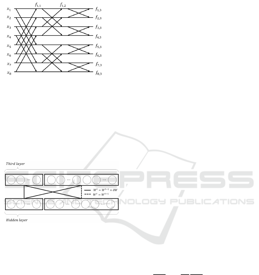
Figure 2: FFT butterﬂy structure.

where f

j,0

has been set equal to x

. To extract the

features at each frequency, we believed that it would

be necessary to use not only the obtained complex

Fourier coefﬁcients, but also all of the f

i,n

values be-

cause it is obvious from Figure 2 that holding f

j,n

in the middle layer enables the extraction of features

from both low and high frequencies.

In our model, we implemented the FFT butterﬂy

structure in the middle layer, which also had the RNN

structure as shown in Figure 3.

Figure 3: Structure of third layer.

When implementing the FFT in this layer, three

points required attention. First, if all of the neurons

had FFT structures, it is conceivable that the learning

would not converge(the dashed line in Figure 3). Sec-

ond, even though the RNN had a mechanism to update

the weights of the connections between the cells (the

solid lines in Figure 3), the weights of the FFT butter-

ﬂy connections weights were constant. Finally, if the

FFT butterﬂy structure had a feedback path to itself

from the RNN, the FFT would not work correctly, as

the inputs were time integrals. This composition is

expected to enable expression of both time and fre-

quency information without losing the RNN’s nature.

2.2 Proposed Model

Our proposed model consists of ﬁve layers, with the

third layer incorporating both the FFT butterﬂy and

RNN structures. Our proposed neural network was

developed based on the deep belief network (DBN)

model (G. E. Hinton and Teh, 2006).

In a DBN, the weights of the network are initial-

ized from the input layer to the output layer by learn-

ing without a teacher as pre-processing for learning.

After that, the weights are updated by using back-

propagation (Hinton and Salakhutdinov, 2006). In

this paper, we set the probability p equal to 0.5 for

drop-out. The ﬁrst and last layers are for the input

and output layers, respectively. Thus, this model has

three middle layers. The second and fourth layers are

normal DBN layers and bind the previous and subse-

quent layers. The only difference between this struc-

ture and that of a normal DBN is in the third layer with

the hidden layer for RNN and FFT butterﬂy struc-

ture. The hidden layer separate from the normal lay-

ers. At time t, the RNN stores the current informa-

tion on the hidden layer after outputting the results.

Next, at time t+1, the hidden layer feeds the informa-

tion corresponding to the previous time back to the

normal layers. Thus, the RNN can learn patterns that

vary with time. We used the equation 2 to perform

forward propagation:

∑

(in)

∑

′

j j

′

t−1

′

. (2)

The indices i and j correspond to the previous

and subsequent layers, respectively, in the RNN; u

is the middle layer input at time t; w

(in)

is the weight

between the input and middle layer; and w

j j

′

is the

weight of the RNN feedback path . The initial value

of w

j j

′

was calculated using autocorrelation, and back

propagation through time was used. The error δ prop-

agated to the previous layer was calculated using the

equation 3. Subsequently, the weight of each connec-

tion was updated using Equation 4.

∑

out

out,t

∑

′

j j

′

t+1

′

(3)

∂E

∂w

j j

′

∑

t=1

∂E

∂u

∂w

j j

′

∑

t=1

t−1

(4)

3 EXPERIMENT

Before controlling a robot with the Tsumori system, it

was necessary to verify the performance of our model.

We expected it to perform well when supplied with

input signals with deviations in their frequency distri-

butions because of the FFT butterﬂy structure. There-

fore, we evaluated the performance of our model

when supplied with signals both with and without de-

viations in their frequency distributions.

BIOINFORMATICS 2016 - 7th International Conference on Bioinformatics Models, Methods and Algorithms

176

3.1 Preparation

To verify the feasibility of using our neural network

model to control a robot, we compared the perfor-

mances of four kinds of neural networks: deep learn-

ing (A), deep learning with FFT butterﬂy (B), RNN

(C), and RNN with FFT butterﬂy (D). The third layer

of model (B) consisted of FFT parts and ordinal neu-

rons for deep learning. All of them have ﬁve layers to

construct the neural network model. The output and

input layers each contained 32 neurons. The second

and fourth layers each had 150 neurons, and the third

layer had 402 neurons. The remaining 352 neurons in

models (B) and (D) also had FFT butterﬂy structures.

We used 32 points for the FFT, with ﬁve butterﬂy op-

erations. We used two neurons to store f

j,n

, which

consisted of real and imaginary parts. The weights

were updated 20 times during the pre-processing of

the Boltzmann machine. In addition, equation 5 was

used as the activation function, where u is the input to

each neuron:

f(u) =

1+ e

−u

(5)

3.2 Performance Veriﬁcation

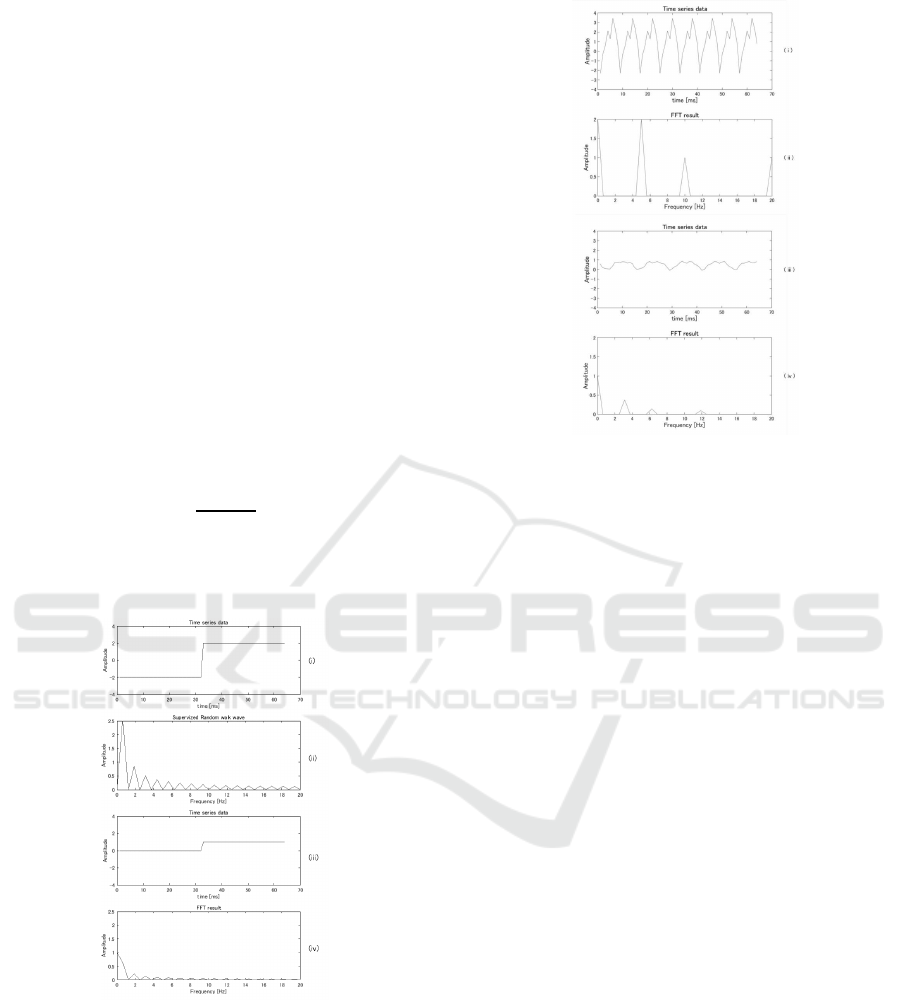
Figure 4: Step function signals.

We veriﬁed the above models from the viewpoint of

frequency distribution. First, we prepared signals that

were uniform in the frequency domain for veriﬁca-

tion. The signals were step functions whose spec-

tra incorporated all of the frequency bands. Figure

6 shows the waveforms and FFT results for the input

and output layers when step function signals with the

form of Equation 6 were applied:

x(t) = au(t − τ) − b (6)

Figure 5: Random walk signals.

In this equation, u(t-) is a step function. The pa-

rameters were set as follows: a = 4, b = 2, andτ = 32

for the input signal, and a = 1, b = 0, andτ = 32 for

the output signal. The signals were fed to the input

layer by shifting them by 1 neuron as time progressed

from t to t + 1. The output data obtained from each

model after 16 steps were used for veriﬁcation.

As step signals are uniform in the frequency do-

main, the implemented FFT structure would not ﬁnd

the structure in the frequency domain. Therefore,

model (A) was expected to perform well when sup-

plied with a step function signal.

The results are shown in Figure 6. In each graph,

the gray lines show the waveforms and frequency dis-

tributions of the supervised data (Figure 4, 5). The

black lines show the results from each model. Model

(A) best reproduced the input data. However, model

(B) could not do so since the almost all of the neurons

in the third layer were employed for the FFT.

The same can be said about model (C). Though the

increases in the signal were identiﬁed by both models,

in model (C), the temporal information about the sig-

nal increases was lost. Model (D) successfully repro-

duced the supplied signal, although it ﬂuctuated. The

frequency distribution generated by model (A) is al-

most identical to that of the original signal, whereas in

the other models, energy leakage is evident. However,

the distribution produced by model (D) is better than

that of model (C) in the low-frequency band. There-

fore, deep learning is the best means of reproducing a

pattern that has a spatial structure, and RNNs cannot

accurately reproduce rising or falling signals. How-

ever, performing an FFT in an RNN could improve

its ability to reproduce such waveforms.

Techniques to Control Robot Action Consisting of Multiple Segmented Motions using Recurrent Neural Network with Butterﬂy Structure

177

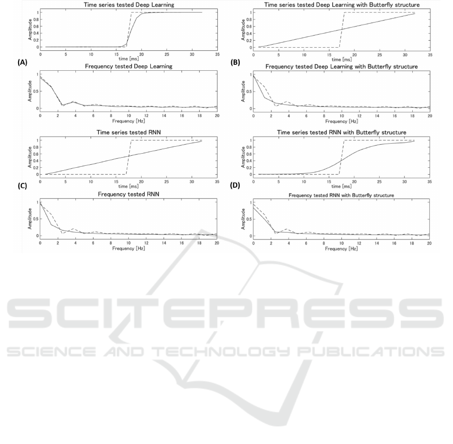
Figure 6: Output from each neural network (step function).

Next, instead of step signals, we used random

walk signals; such signals have variations in their

frequency distributions. In the real world, signals

with uniform frequency distributions, such as step sig-

nals, are few. Instead, most signals have biased fre-

quency distributions, like those of random walk sig-

nals. Therefore, it was reasonable to use these to

verify the abilities to reproduce the signals by using

FFTs. The signals had the following form (Tachi,

1993):

x(t) =

∑

k=1

−k

sin2π f

min

t + φ

). (7)

The parameters were set as follows: a

= 2, p =

2, n = 3, and f

min

= 5 for the input signal, and a

20, p = 2, n = 3, and f

min

= 3 for the output supervised

signal. The amplitudes of both the input and output

signals were inversely proportional to the frequency

from Equation 5. Hence, the energies of the signals

at each frequency and the velocity amplitudes were

constant, and the sine wave at each frequency was in-

dependent of φ

and the sampling frequency was 40

Hz. The waveforms and FFT results for the input and

output layers when supplied with random walk sig-

nals are shown in Figure 7. Graphs (i) and (ii) cor-

respond to the input signal, and graphs (iii) and (iv)

correspond to the supervised.

Figure 7 shows the results. Ideally, the waveforms

obtained by the neural network would have peaks in

the frequency domain at 3 Hz, 6 Hz, or 12 Hz. Models

(A) and (B) show no marked differences, regardlessof

the presence of the FFT butterﬂy. In the FFT results

for these two models, the energies of the signals at

each frequency were largely lost.

Model (B) failed to reproduce the waveform and

frequency distribution of the signal. The reason for

this failure is believed to be that, as this model had

no recurrent structure, it could not identify the time-

varying components of the signal. Although model

age occurred across a wide frequency range, and it

was very difﬁcult to estimate the original waveform

from the measured one. On the other hand, the out-

put from model (D) has peaks at 3 Hz and 6 Hz in the

FFT results. Although there is no peak at 12 Hz, the

energy is not zero. Therefore, it is said that model (D)

best reproduced the original waveform.

3.3 Tsumori by RNN with FFT

Next, we used our model to control a robot through

the Tsumori framework, as the inputs of the Tsumori

system have temporal continuity and contain multi-

frequency information. The sampling frequency was

40 Hz, and each segmented robot action was de-

scribed with 64 units in the Tsumori system. We

asked one subject to generate inputs using the con-

trol stick based on the robot’s action, such as raise its

hands” with the intention, ”I move this robot”. This is

a basic operation required to enable a robot to lift an

object and is applicable to many situations. The sub-

ject repeated this operation 10 times; the ninth data

BIOINFORMATICS 2016 - 7th International Conference on Bioinformatics Models, Methods and Algorithms

178

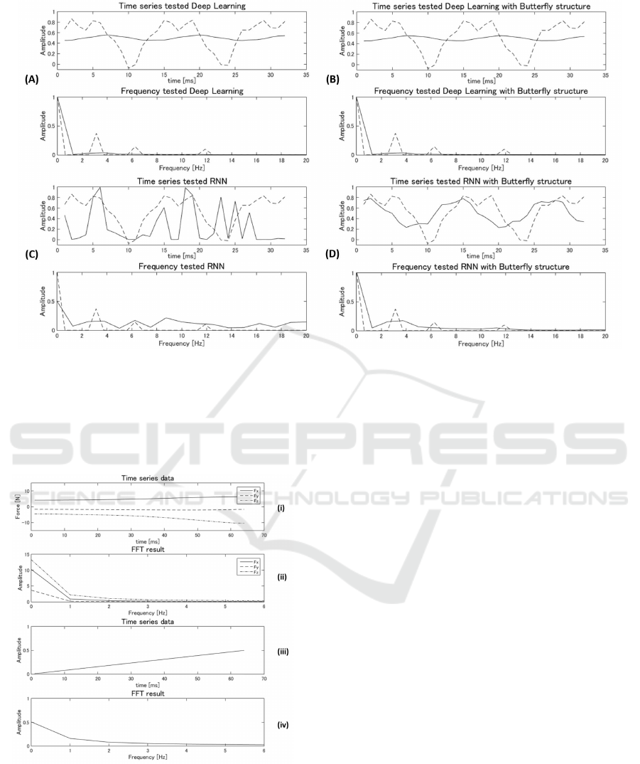
Figure 7: Output from each neural network (random walk).

set was used for learning, and the 10th was used to

test the neural network. Figure 8 shows the wave-

forms and FFT results corresponding to the input by

the subject and the actual movement of the robot servo

motor.

Figure 8: Operator input.

In Figure 8, (i) and (ii) show only three DOFs, the

forces along the three axes, and (iii) and (iv) corre-

spond to just the pitch of the right shoulder. In fact,

the operator inputs had 12 DOFs, which consisted of

forces along and moments about the three Euclidian

axes for both hands. In this study, six DOFs were

used in total because the inputs from the operator’s

two hands were considered to be symmetrical. Fur-

thermore, the number of DOFs of the robot’s upper

limbs was reduced from six to three: the roll and pitch

of the right shoulder and the pitch of the right elbow.

In this experiment, a KHR3HV robot was controlled

by the Tsumori system.

Some changes were made to the neural network to

apply it to the Tsumori system. We prepared 192 neu-

rons for the input layer and 96 for the output layer, be-

cause the operator input consisted of six DOFs, while

the robot had only three DOFs. A total of 1000 neu-

rons for the second layer, 600 for the fourth layer, and

2262 neurons for third layer were prepared. In the

third layer, 2112 neurons had FFT butterﬂy connec-

tions and the remaining 150 neurons were used for

the RNN. In this experiment, the neural networks re-

ceived operator inputs corresponding to two motion

segments for the robot. Therefore, 32 pieces of data

were input simultaneously, corresponding to a total of

64 with one DOF each, and each piece of data was

recorded in a separate time interval. Therefore, the

time varied from 0 and 63. As Figure 9 shown, the re-

sulting frequency distribution and waveform are both

quite similar to those of the original signal.

4 DISCUSSION

For the step function signals, model (A) best repro-

duced the original signals, because the deep learning

Techniques to Control Robot Action Consisting of Multiple Segmented Motions using Recurrent Neural Network with Butterﬂy Structure

179

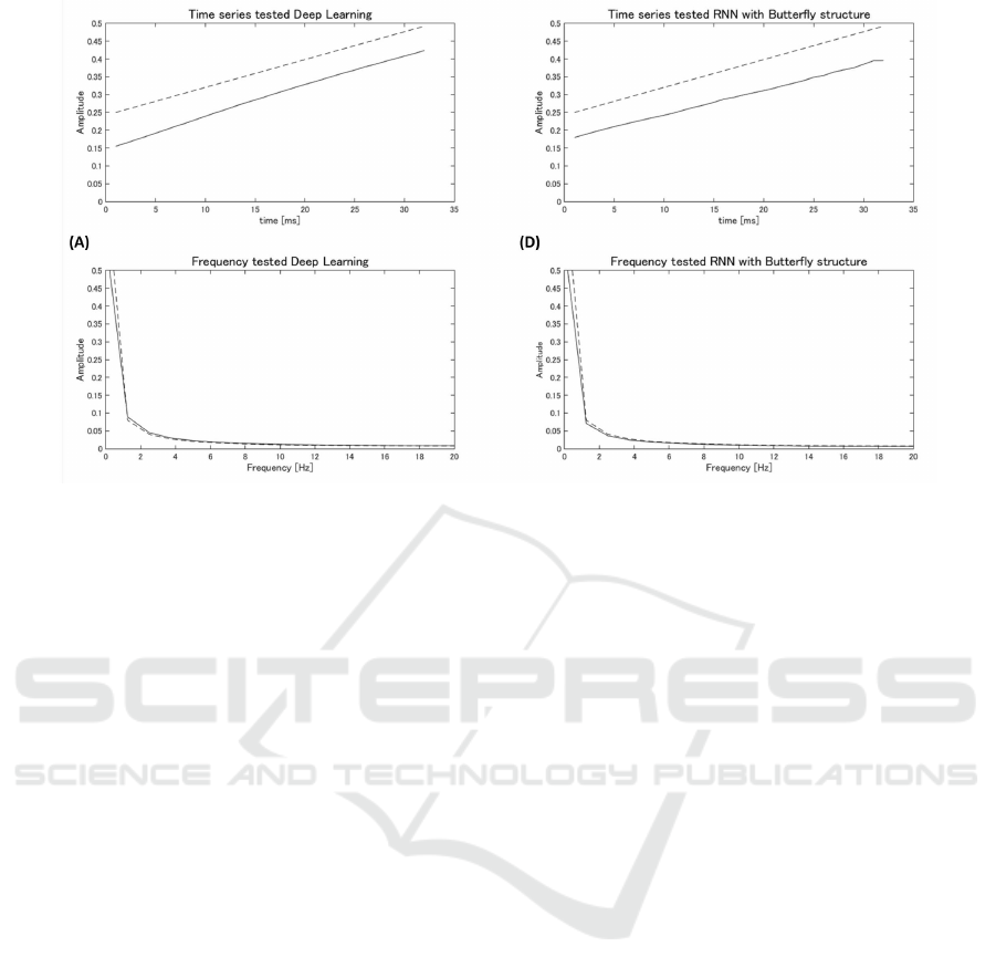
Figure 9: Output Tsumori system output.

method can accurately determine spatial structures.

For this reason and because the rising of the signal

appeared locally, it was considered that model (A) re-

membered only that information. On the other hand,

although some of the structure of model (B) was the

same as that of model (A), the waveform was lost be-

cause the FFT result for the step signal contained less

information (from Figure 4) and the number of neu-

rons for deep learning was lower than that of model

(A). Model (C) also could not reconstruct the wave-

form. Although an RNN can accurately reproduce

time-varying data, the learning process was ineffec-

tive, as the change was local. On the other hand, the

waveform and frequency distribution were both well

reproduced by model (D) by performing an FFT. The

FFT did not provide information about the energy, but

it did yield information about the phase of each fre-

quency. From this information, the RNN could ﬁnd

the change in the time domain.

Next, we compare the performances of the models

when random walk signals were applied. Models (A)

and (B) could not reproduce the random walk wave-

forms, as deep learning cannot identify the features

of time-varying data. In model (B), though the FFT

provided frequency information, it lacked the infor-

mation about the temporal variations. The results of

model (C) were the worst of all the models, however,

upon implementing the FFT structure, model (C) be-

came the best model. Except for the energy leakage

at lower frequencies, model (C) maintained the en-

ergy of the entire system. Accordingly, RNNs might

enable complete reproduction of frequency informa-

tion if the energy leakage problem can be solved.

Two problems related to energy leakage were con-

sidered. First, the recursion times of the RNN were

few to converge to the optimal network. In this study,

the recursive method of the RNN was employed only

once. It is conceivable that the energy leakage would

decrease by performing the RNN method repeatedly.

Another problem was that the temporally continuous

data we used were long for the RNN. Therefore, the

RNN might not have been able to remember old in-

formation about the weights of the connections. To

solve this problem, it might be beneﬁcial to imple-

ment a long short-term memory (LSTM) (Hochreiter

and Schmidhuber,1997) structure or more hidden lay-

ers than were used in this model.

Finally, we compare the robot control signals of

the Tsumori framework. Both models (A) and (D)

produced waveforms and frequency distributions sim-

ilar to those of the original data. It is believed that

model (A) could learn the spatial features of the sig-

nal since it was monotonous. However, as shown in

the results corresponding to the random walk signals,

model (A) failed to reproduce the signals if they con-

sisted of multiple frequencies. Our objective in this

research was to enable robot control based on input

consisting of multiple operator intentions; therefore,

it is necessary to verify the performances of robots

when given such inputs.

5 CONCLUSION

This paper introduced a new deep-learning model for

learning signals consisting of multiple frequencies,

BIOINFORMATICS 2016 - 7th International Conference on Bioinformatics Models, Methods and Algorithms

180

and its ability to reproduce the original signals was

discussed by comparing its performance with those

of the existing models. We also experimentally veri-

ﬁed its practicality for robot control by using operator

inputs applied through the Tsumori framework. Our

approach yielded the optimum results for determining

information in the frequency domain when an RNN

with an FFT structure was used. The results indicate

that a neural network with RNN and FFT butterﬂy

structures could learn data consisting of multiple fre-

quencies. This corresponds to a robot learning an ac-

tion consisting of multiple segments. Therefore, this

neural network can be used to construct learning ma-

chines that associate multiple operator intentions with

robot actions in the Tsumori framework. In the future,

we plan to verify the ability of this model to produce

robot movements when presented with multiple seg-

mented operator intentions through the Tsumori ar-

chitecture. These inputs will resemble the random

walk signals used in this study.

ACKNOWLEDGEMENTS

This work was funded by the ImPACT Program of

the Council for Science, Technology and Innovation

(Cabinet Ofﬁce, Government of Japan). It was also

supported by Osaka University, Institute for Aca-

demic Initiatives, Division 4, Humanware Innovation

Program and a JSPS KAKENHI Grant-in-Aid for Sci-

entiﬁc Research (A), Grant Number 15H01699.

REFERENCES

Ando, H., Niwa, M., IIzuka, H., and Maeda, T., editors

(2012). Effects of observed motion speed on segment-

ing behavioural intention.

G. E. Hinton, S. O. and Teh, Y. (2006). A fast learn-ing

algorithm for deep belief nets. Neural Computation,

18(2):1527–1544.

Hinton, G. E. and Salakhutdinov, R. (2006). Reducing the

dimensionality of data with neural networks. Science,

313:504–507.

Hirai, K., Hirose, M., Haikawa, Y., and Takenaka, T., ed-

itors (1998). The Development of Honda Humanoid

Robot, volume 2. IEEE.

Hochreiter, S. and Schmidhuber, J. (1997). Long short-term

memory. Neural Computation, 9(8):1735–1780.

Le, Q., Ranzato, M. A., Monga, R., Devin, M., Chen, K.,

Corrado, G., Dean, J., and Ng, A., editors (2012).

Building high-level features using large scale unsu-

pervised learning.

Mikolov, T., Kombrink, S., Burget, L., Cernocky, J., and

S.Khudanpur, editors (2011). Recurrent Neural Net-

work Based Language Model.

Niwa, M., S.Okada, Sakaguchi, S., Azuma, K., Iizuka, H.,

H, A., and Maeda, T., editors (2010). Detection and

Transmission of Tsumori : an Archetype of Behav-

ioral Intention in Controlling a Humanoid Robot.

Yamamoto, T. and Fujinami, T. (2004). Synchronisation

and differentiation: Two stage of coordinative struc-

ture. In Third International Work-shop on Epigenetic

Robotics, pages 97–104.

Techniques to Control Robot Action Consisting of Multiple Segmented Motions using Recurrent Neural Network with Butterﬂy Structure

181