Geometry Analysis of Superconducting Cables for the Optimization of

Global Performances

Nicolas Lermé

1,2∗

and Petr Dokládal

MINES ParisTech, PSL Research University, Centre for Mathematical Morphology, Fontainebleau, France

Institut d’Électronique Fondamentale, Université Paris-Sud, Gif-sur-Yvette, France

Keywords:

Segmentation, Registration, Shape Analysis, Clustering, Superconductivity, Cable.

Abstract:

Superconducting cables have now become a mature technology for energy transport, high-ﬁeld magnets (MRI,

LHC) and fusion applications (ToreSupra, and eventually ITER and DEMO). The superconductors are ex-

tremely brittle and suffer from electrical damages brought by mechanical strain induced by electromagnetic

ﬁeld that they generate. An optimal wiring architecture, obtained by simulation, can limit these damages.

However, the simulation is a complex process and needs validation. This validation is performed on real 3D

samples by the means of image processing. Within this objective, this paper is, to our best knowledge, the

ﬁrst one to present a method to segment the samples of three types of cables as well as a shape and geometry

analysis. Preliminary results are encouraging and intended to be later compared to the simulation results.

1 INTRODUCTION

1.1 Motivation and Scope

Superconducting cables have now become a mature

technology in energy transport, high-ﬁeld magnets

(medicine (MRI), high-energy physics (LHC)) and

magnetic conﬁnement in fusion applications (Tore-

Supra, eventually ITER and DEMO reactors).

A superconducting cable presents a multiscale in-

ternal structure. Such a cable consists of strands ar-

ranged together given some application-dependent ar-

chitecture. Individual strands are composite struc-

tures either formed by superconducting microﬁla-

ments embedded in a metallic matrix or a thin super-

conducting layer deposited onto a metallic substrate.

A substantial drawback of some of these cables

is the fragility of the superconductors. Mechanical

strains can indeed cause deformations, thus degrading

their performance.

Whereas these strains can be limited during shap-

ing (wiring or winding) or thermal cool-down, they

remain problematic during operation when exposed

to high electromagnetic ﬁelds due to its own Lorentz

∗

This work was funded by the ANR project ANR-

GUI-AAP-05 (2013–2017) and performed during the post-

doctoral research project of Nicolas Lermé at the Centre for

Mathematical Morphology.

force (particularly under cyclic loading).

However, the performance degradation can be di-

minished by optimizing the geometry of the cables.

Optimize the performance of these cables is thus es-

sential and could directly beneﬁt to a large number of

research and industrial actors.

The global performances of the cable are simu-

lated using models of the electrical and/or mechani-

cal behavior of the cable structure (Torre et al., 2014;

Manil et al., 2012). Given the complexity of vari-

ous types of cables, the validation of these models

is done by statistical comparison of the geometry of

the models to the geometry of real cables obtained

from tomography images. Depending on the result of

these comparisons, the design of the cables can be op-

timized, until a better cable architecture is obtained.

This paper focuses on the identiﬁcation of the

experimental geometry on three types of cables, in-

volving mostly

automatic registration, segmenta-

tion, clustering and features extraction tasks. To our

best knowledge, this is the ﬁrst paper providing meth-

ods and results for the geometry analysis on these ca-

bles. For each type of cable, we provide below the

physical parameters and the image characteristics.

The method for segmenting cables-in-conduit is semi-

automatic since initial manual markers are required.

540

Lermé, N. and Dokládal, P.

Geometry Analysis of Superconducting Cables for the Optimization of Global Performances.

DOI: 10.5220/0005667105400551

In Proceedings of the 5th International Conference on Pattern Recognition Applications and Methods (ICPRAM 2016), pages 540-551

ISBN: 978-989-758-173-1

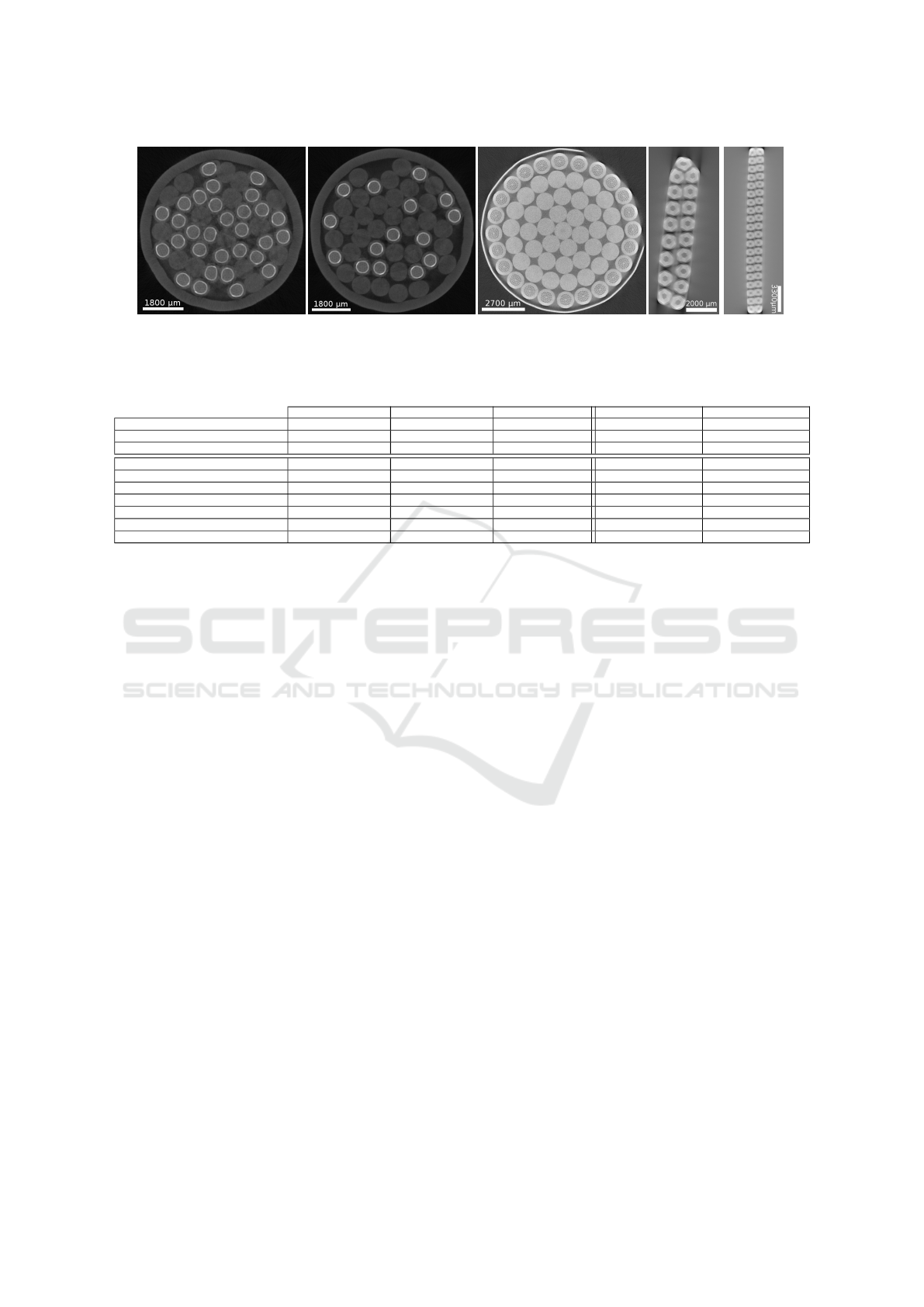
(a) N05 (b) N22 (c) mgb2_113 (d) 18RRPN01 (e) 40RRPR02

Figure 1: Cross-sectional images from cables-in-conduit (a,b), power cables (c) and Rutherford cables (d,e).

Table 1: Image characteristics (top) and physical parameters (bottom) of the cables-in-conduit (left to the double bar) and

power cables (right to the double bar).

N05 N22 N25 mgb2_113 mgb2_133

Image size (x, y,z)

750 ×800×12431 750×850×12424 750 ×750×7745 1200 ×1200×5972 1300 ×1605×6071

Resolution (µm)

12 12 12 10 10

Memory usage (GB)

6.94 7.37 4.05 8.1 12

Number of s.c./n.s.c. (all) strands

30/15(45) 15/30(45) 30/15(45) 24/37(61) 24/37(61)

Strand  (µm)

800 800 800 1130 1330

Avail. sample length (µm)

149172 149088 92940 59270 60710

Twist-pitch sequence (mm)

45/85/125 45/85/125 35/65/110

227 260

First triplet (s.c.,n.s.c.)

(2,1) (1,2) (2,1)

/ /

Cable pattern

(3,3,5) (3,3,5) (3,3,5)

/ /

Void fraction (%)

25 33 33 24.7 24.7

1.2 Available Cables

Three distinct types of cables are considered with

different architectures, appearances and composition:

the cables-in-conduit (Weiss et al., 2007), the Ruther-

ford cables (Oberli, 2013; Milanese et al., 2012)

and the power cables (Seidel and Sturge, 2009; IEC,

2004). Several samples of each with different param-

eters were analyzed (see Tab. 1 and 2 for their charac-

teristics, and Fig. 1 to assess the variety and the qual-

ity of the images).

Cables-in-conduit (see Fig. 1(a,b)) consist of su-

perconducting strands (s.c.) and non-superconducting

strands (n.s.c.). S.c. strands are composed of kernels

in Nb

Sn and bronze (white) wrapped by a jacket in

copper (gray) while n.s.c. strands are made of copper

(gray). All strands are twisted together in a multistage

fashion according to a predeﬁned cable pattern com-

posed of stages and petals. For instance, the pattern

(3,3,5) of the cable N05 has three stages. The ﬁrst

(lower) stage consists of twisted triplets (15 petals),

each with 2 s.c. and 1 n.s.c. strands. These triplets

are again twisted by three (5 petals) and ﬁnally by

ﬁve (1 petal), thus leading to a total of 30 s.c. and

15 n.s.c. strands. All strands are then inserted in a

stainless steel conduit. Some void fraction is kept to

enable the circulation of a cooling ﬂuid (helium). No-

tice that all stages are twisted with a different twist-

pitch. Typically used in fusion applications, these ca-

bles can transport currents of 45kA under a magnetic

ﬁeld of 12.3T, exposed to transversal Lorentz forces

of 554kN/m.

Power cables (see Fig. 1(c)) consist of s.c. strands

in MgB

/nickel alloy and n.s.c. copper strands. All

strands are arranged in concentric layers, twisted and

inserted in a corrugated cryogenic envelope. Again,

some void fraction is kept to enable the circulation of

a coolant (gaseous and eventually liquid helium). S.c.

strands are located on the outer layer. Typically used

in energy distribution, each strand can convey a cur-

rent of 400A under a magnetic ﬁeld of 1T, developing

radial, centripetal, Laplace forces of 400N/m.

Rutherford cables (see Fig. 1(d,e)) roughly consist

of s.c. strands composed of cores in copper (gray) sur-

rounded by an intermediary zone containing Nb

ﬁlaments (white), themselves wrapped in a copper

jacket (gray). All strands are twisted to form a two-

layers ﬂat cable, compressed to a well-controlled rect-

angular section. Depending on the design used, the

ﬁlaments zone is arranged to form either an hexagon

or a circle. Typically used in medical imaging and

high-ﬁeld magnets, these cables can transport cur-

rents of the order of 20kA under a magnetic ﬁeld of

10 −15T, exposed to Lorentz forces of 1−5MN/m.

1.3 Outline of the Paper

The rest of this paper is as follows. In Section 2, we

brieﬂy explain the registration of overlapping sam-

ples. In Section 3, we detail, for each type of cable,

the proposed methods for extracting the structures of

interest from the resulting images. In Section 4, we

Geometry Analysis of Superconducting Cables for the Optimization of Global Performances

541

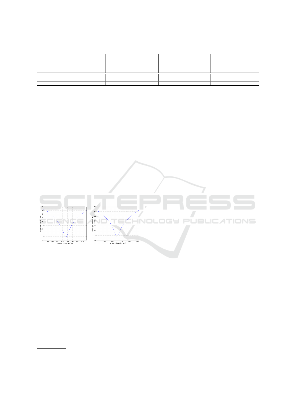
Table 2: Image characteristics (top) and physical parameters (bottom) of the Rutherford cables.

COP-RRP 18PITN01 18PITN01_2 18RRPN01 18RRPN01_2 40RRPR01 40RRPR02

Image size (x, y,z)

1500 ×

300 ×1300

750 ×

1100 ×1200

1600 ×500 ×

1200

1100 ×

750 ×1200

1700 ×700 ×

1200

1600 ×

500 ×1200

1500 ×

500 ×1200

Resolution (µm) 15 10 6.75 10 6 15 15

Memory usage (MB) 558 945 916 945 1434 916 859

Number of strands 40 18 18 18 18 40 40

Strand  (µm) 1050 1020 1000 1050 1046 1080 1035

Avail. sample length (µm) 19500 12000 8100 12000 7200 18000 18000

propose indicators reﬂecting potential damages. Fi-

nally, we present results in Section 5 and discuss fu-

ture work in Section 6.

2 IMAGE REGISTRATION

The cable samples being too long to be imaged at

once, multiple overlapping scans have been acquired

with a constant translation step along the z-axis

Each scan has then been registered on the previous

one by minimizing the Mean Square Error (MSE) of

the difference of intensities over the overlapping re-

gion along the z-axis. The minimization along the z-

axis is sufﬁcient since no residual displacement along

the x and y axes was observed. The Fig. 2 depicts the

MSE as a function of the varying overlap between two

successive scans, for a cable-in-conduit (N05) and a

power cable (mgb2_113).

Figure 2: MSE of two overlapping scans for a cable-in-

conduit (left) and a power cable (right).

3 IMAGE SEGMENTATION

The purpose of the segmentation is to extract the con-

tours of strands (and the conduit, if need be) and their

centerlines. Most structures to extract are nearly cir-

cular and touch each other. Their appearance and con-

trast however differ for all cable architectures. Dis-

tinct algorithms have been designed for all types of

cables with their own set of parameters. Some of

these parameters still require a manual tuning (in this

case, it will be mentioned below). However, most of

them appear to be stable and expressed with respect

to the image resolution and cables characteristics.

From here, the z-axis will refer to the longitudinal one

while x,y axes will refer to transversal ones.

These algorithms share common difﬁculties to

overcome to get reliable measurements. First, they

must be able to assess slight deviations from the cir-

cularity, be robust to noise, artifacts and poor contrast.

Second, they must be fast and able to handle large vol-

ume data (possibly more than shown in Tab. 1 and 2).

To accommodate these constraints, a simple approach

has been preferred (whenever possible) where the 3D

volume is segmented as a sequence of 2D images

along the z-axis. This allows to run some steps in par-

allel. Once strand contours have been obtained, the

centerlines consist of the strand centroids. Moreover,

we assume the following known and constant: the di-

ameter of a strand (denoted by S

), the thickness of

the strand jacket (denoted by S

), the thickness of the

conduit of the cable (denoted by C

) as well as the

number of s.c. and n.s.c. strands (denoted by N

and

nsc

, resp.).

3.1 Rutherford Cables

The core of strands being better contrasted than the

jackets, we propose an automatic procedure that relies

on the ﬁlaments zone to extract the contours of strands

in two steps (see Fig. 3).

3.1.1 Extraction of Cores

First, an Alternate Sequential Filter (ASF) is applied

on the source image with a squared structuring ele-

ment up to the size of 0.03 ×S

(Sternberg, 1986)

(image I

(a)). This allows us to both denoise the im-

age and ﬁll the interstices between ﬁlaments. Next, a

ﬁlling algorithm is applied on the image I

(image

(b)). The image I

is then subtracted from the

image I

(image I

(c)). Once the image I

thresh-

olded (image I

(d)), it both contains cores and in-

terstices. To discard the interstices, a mask is built

by thresholding the image I

(image I

(e)) and ap-

plying a morphological erosion with a square of size

0.15 ×S

as structuring element (image I

(f)). Fi-

nally, the mask I

is intersected with the image I

and

the 3D N

largest connected components are kept.

The resulting components are labeled and correspond

to the cores (image I

(g)). Due to the variety of im-

ages, notice that the above thresholds need to be man-

ually adjusted, independently of ground truths (see

Section 5.1.1).

ICPRAM 2016 - International Conference on Pattern Recognition Applications and Methods

542

(a) I

(b) I

(d) I

(e) I

(f) I

(g) I

(h) I

(α = 10

) (i) I

(α = 0) (j) I

(α = 10

) (k) I

(α = 10

) (l) I

Figure 3: Steps for extracting the cores (a-g) and the strands (h-l) from an image of a Rutherford cable (COP-RRP). The source

image is ﬁrst denoised by an ASF (a). Once (a) ﬁlled (b), it is subtracted from (a), giving (c). An intermediate result (d) is

obtained by thresholding (c). A mask (f) is built by thresholding (b) (giving (e)) and applying a morphological erosion on the

result (f). (f) is then intersected with (d) and the 3D N

largest connected components are kept. The resulting components

are labeled and correspond to the cores (g). A region-growing algorithm is then used to extract the ﬁlaments zone, based on

geodesic distance maps whose amount of regularity is controlled by a parameter α (h). The impact of α after region-growing

is shown when it is small (i), moderate (j), large (k). The strands are obtained by expanding the ﬁlaments zone with α = 0 (l).

3.1.2 Extraction of Strands

As shown in Fig. 3, the ﬁlaments zone is poorly con-

trasted and strands touch with each other. To over-

come these difﬁculties, we introduce several priors

(near circularity, small displacement and volume con-

servation of strands sections) and proceed in two suc-

cessive steps.

First, a distance transform is computed from each

labeled core of I

using an efﬁcient pixel queue al-

gorithm (Ikonen, 2005). This algorithm has a worst-

case complexity of O(n log n) (where n is the number

of pixels in the image). Each distance map is com-

puted using the WDTOCS metric, described in (Iko-

nen, 2005). Let I : Ω ⊂ Z

→ R be an image and

N be a neighborhood. Without loss of generality, we

propose to use

N = {(p,q) ∈ (Ω ×Ω) | kp −qk ≤

√

2},

where k.k is the L

norm in Z

. For any pair (p, q) ∈

N , the WDTOCS metric is deﬁned as

dist(p, q) =

kp −qk

+ α(I

−I

)

, (1)

where α ∈ R

is a parameter that balance geometric

and image information. The larger the parameter α

is, the more the image information is taken into ac-

count. An example of distance map from the right-

most core is shown in (h) where the distance is pro-

portional to the intensity (the dynamic of the image

has been stretched for visualization purpose). Dis-

tance transforms being independent from each other,

their computation is in practice performed in parallel

using OpenMP. Once all the distance maps obtained

using α > 0, a region-growing algorithm is applied

to obtain the outer contour of the ﬁlaments zones: all

cores grow simultaneously by greedily selecting the

pixels having the minimum cost based on their respec-

tive distance maps, until a target volume is reached

The effect of varying the parameter α after region-

growing is depicted on the image I

when α is small

(i), moderate (j) and large (k). Finally, the contours of

strands are obtained by expanding the ﬁlaments zones

in such a way that none of them is favored. This is

achieved by repeating the above steps for α = 0 (im-

age I

(l)). In our experiments, we set α = 10

3.2 Cables-in-conduit

As shown in Fig. 4, the s.c. strands are better con-

trasted than the n.s.c. ones. Based on this observation,

we propose a three-steps scheme that ﬁrst extracts au-

tomatically the conduit and then the s.c. strands. The

n.s.c. strands are then semi-automatically extracted

based on initial markers.

3.2.1 Extraction of the Conduit

First, the source image is denoised by an ASF with a

squared structuring element up to the size of 0.05 ×

(Sternberg, 1986) (image I

(a)). To further ﬂat-

ten homogeneous areas, the image I

is ﬁltered by a

Gaussian of size 0.05 ×S

and thresholded (image

(b)). Next, a morphological opening, a holes ﬁlling

algorithm and then a morphological closing are ap-

plied on the image I

using a square of size 0.2 ×S

as structuring element (image I

(c)). Assuming the

ideal conduit is nearly circular, an ellipse is ﬁtted on

the image I

. Its size is subtracted by 2×C

to ﬁt the

inner contour of the conduit (image I

(d)).

It is adjusted if the ﬁlaments zone is an hexagon.

Geometry Analysis of Superconducting Cables for the Optimization of Global Performances

543

(a) I

(b) I

(d) I

(e) I

(f) I

(g) I

(h) I

(i) I

(j) I

(z = 0) (k) I

(z = 6211) (l) I

(z = 12423)

Figure 4: Steps for segmenting the conduit (a-d), the s.c. strands (e-h) and the n.s.c. strands (i-l) from an image of a cable-in-

conduit (N22). The source image is ﬁrst denoised by an ASF (a). Next, (a) is ﬁltered by a Gaussian and thresholded (b). Holes

are ﬁlled in (b) by various morphological operations (c). An ellipse is then ﬁtted on (c) and adjusted on the inner contour of

the conduit (d). Once the conduit obtained, (a) is thresholded from the source image (e), dilated and ﬁlled (f). Using (d) and

(f), kernels are obtained by applying a watershed algorithm (g) on the source image. S.c. strands (h) are then extracted by

expanding (g) (same approach as Rutherford cables with α = 0) and subtracting the complement of (d). Finally, n.s.c. strands

are extracted with α > 0 (j-l), constrained by (d) and (h) but from the strands centroids f the previous image (i).

3.2.2 Extraction of the S.C. Strands

The strategy employed here is to rely on kernels to ex-

tract the contours of strands. For doing so, the source

image is ﬁrst thresholded (image I

(e)). Next, the

resulting contours are closed using a morphological

dilation with a square of size 0.25×S

as structuring

element and holes are ﬁlled (image I

(f)). To prop-

erly align the segmentation on the contours of kernels,

a watershed algorithm (Meyer, 1991) is applied on the

source image (image I

(g)). The outside marker is

the complementary of the image I

and the markers

representing the kernels are obtained by performing a

morphological erosion of the image I

with a squared

structuring element of size 1.25 ×S

. As for Ruther-

ford cables, s.c. strands are ﬁnally obtained by ex-

panding the kernels from the image I

with α = 0

(see Section 3.1.2) and subtracting the complement

of the mask I

(image I

(h)).

3.2.3 Extraction of the N.S.C. Strands

To overcome the poor contrast on n.s.c. strands,

we adopt the same strategy as for Rutherford cables

(see Section 3.1.2) but with two differences. First,

the geodesic distances are computed using α > 0

but constrained in I

. Second, the centroids of

s.c. strands must be provided as initialization (image

(i)). Geodesic distance maps are computed from

these centroids and the region-growing algorithm is

applied. Once the centroids computed on the result-

ing contours of strands, the same procedure is applied

on the next image (image I

). This process contin-

ues until the end of the cable is reached. To illustrate

the correctness of the propagation, the image I

shown with the n.s.c. strands obtained at the begin-

ning (j), the middle (k) and the end (l) of the cable.

Unlike Rutherford cables, it is important to notice that

such an approach can fail to recover the contours of

n.s.c. strands since centroids depend on the result of

the previous image. Such a situation can occur when

the contribution of the right term in Eq. 1 is insuf-

ﬁcient. In that case, the procedure becomes unable

to stick to the contours of strands. A suitable value of

the parameter α must therefore be chosen carefully. In

our experiments, we have chosen to set α = 8 ×10

3.3 Power Cables

For extracting strands, a convenient solution would be

to use the same approach as for Rutherford cables (see

Section 3.1.2) and for the n.s.c. strands of the cables-

in-conduit (see Section 3.2.3). As shown in Fig. 1,

despite the important amount of noise, the images of

power cables present however a much better contrast

compared to the images of the other types of cables.

We detail below a simple procedure that automatically

ﬁnd the contours of the conduit and then the strands,

both assumed to be nearly circular.

First, the source image is thresholded (image I

(a)) and holes are ﬁlled (image I

(b)). From the

image I

, the largest connected component is dis-

carded and a morphological opening is applied with

a squared structuring element of size 0.1×C

(image

(c)). An ellipse is then ﬁtted on the image I

. Its

size is subtracted by C

to ﬁt the inner contour of the

conduit (image I

(d)).

Second, the source image is denoised by an ASF

with a squared structuring element up to the size of

0.05 ×S

(image I

(e)) (Sternberg, 1986). A ﬁrst

rough estimate of the contours of strands is obtained

by thresholding the image I

(image I

(f)). The

ICPRAM 2016 - International Conference on Pattern Recognition Applications and Methods

544

(a) I

(b) I

(d) I

(e) I

(f) I

(g) I

(h) I

(i) I

(j) I

(k) I

(l) I

Figure 5: Steps for segmenting the conduit (a-d) and the strands (i-l) of a power cable (mgb2_113). First, the source image is

thresholded (a) and ﬁlled (b). From (b), the largest connected component is discarded and a morphological opening is applied

(c). An ellipse is ﬁtted on (c) and adjusted on the inner contour of the conduit (d). Second, the source image is denoised by

an ASF (e) and thresholded (f). The complement of (d) is subtracted from (f) and a morphological opening is applied (g). 3D

connected components that do not spread all along the cable are removed (h). The Euclidean distance to the contours of (h)

is computed, ﬁltered (i) and maxima are identiﬁed (j). Strands contours are obtained by applying a watershed (l) on an image

(k) combining the morphological gradient of the source image and the inverted distance map to ideal contours from maxima.

complement of the mask I

is then subtracted from

the image I

and a morphological opening is applied

with a square of size 0.03×S

as structuring element

(image I

(g)). Next, 3D connected components that

do not spread all along the cable in the background

are removed (image I

(h)). From the image I

, the

Euclidean distance to the contours is computed and

the resulting image is ﬁltered by a Gaussian of size

0.25 ×S

(image I

(i)) to ensure a good detection

of maxima (image I

(j)). Finally, the contours of

strands are obtained by applying a watershed (Meyer,

1991) performed on the summed image I

(k) com-

posed of the inverted distance map to ideal contours

from maxima and the morphological gradient (multi-

plied by a factor set to 0.1) of the source image (image

(l)). The multiplier ensures the strands sections to

remain mostly circular along the cable.

4 DAMAGE INDICATORS

During operation, the cables can be exposed to

transversal Lorentz forces up to several MN/m. These

forces induce deformation and/or damages to strands

that come out as various geometrical features. The

features detailed below aim at detecting these defor-

mations.

4.1 Strand Section Compression

Any deviation to the circularity of strands is a poten-

tial source of damage that need to be measured. A

variety of shape descriptors has been proposed in the

literature. In this setting, desirable properties of shape

descriptors are the invariance to translation and rota-

tion, the robustness to noise and a reasonable sensitiv-

ity. The papers (Montero, 2009; Žuni

c, 2012) gather

a large number of descriptors, out of which two have

been selected as applicable in this context and of-

fering similar performance. Let S ⊂ Z

be a strand

section of a 2D binary image taken along the z-axis.

These two descriptors are deﬁned as follows:

EF(S) =

max

min

∈ [1,+∞[ (Elongation Factor),

where λ

min

, λ

max

are the eigenvalues of the covariance

matrix of the strand section S, and

CMPN(S) =

(]S)

2π(µ

2,0

+ µ

0,2

)

∈]0,1] (Compactness),

where ] denotes the cardinality of a set and µ

p,q

de-

notes the moment of order (p + q) of the strand sec-

tion S. EF and CMPN are statistical descriptors. EF

is lower-bounded by one for a circle and increases

for elongated shapes while CMPN is upper-bounded

by one for a circle and tends to zero for elongated

shapes. These two descriptors verify the above men-

tioned properties.

4.2 Curvature

For all the considered types of cables, strands can lo-

cally bend signiﬁcantly and these locations are poten-

tially source of damage. Do detect bendings with a

large amplitude, we propose to measure the local cur-

vature of the strand centerlines.

The curvature measures a failure of a curve to be

straight. It is is positive or null and equal to the in-

verse of the radius of the tangent circle.

Let us represent a centerline with a two times

continuously differentiable space curve C (t) =

(x(t),y(t),z(t))

∈ R

, parameterized by t. Also, we

Geometry Analysis of Superconducting Cables for the Optimization of Global Performances

545

denote resp. by γ

(t) and γ

(t) the ﬁrst and second and

derivatives of C with respect to t. The local curvature

of the curve C is deﬁned by

κ(t) =

kγ

(t) ×γ

(t)k

kγ

(t)k

, (2)

where k.k and × are respectively the L

norm and

the cross product, both in R

. In what follows, we

brieﬂy discuss some numerical considerations. First,

to avoid division by zero, Eq. 2 is set to zero when

the denominator is smaller than some ε > 0

. Sec-

ond, the derivatives are approximated by standard ﬁ-

nite central differences. Due to the presence of noise,

estimating small values of curvatures is however a

delicate problem. Nevertheless, under the assump-

tion that the strands cannot mechanically bend over

some limit value, the ﬁnite differences are computed

using a grid spacing (denoted by ∆h) proportional to

the strand diameter S

. A large value of ∆h allow

us to assess small curvature values despite the noise.

Also, we choose not to consider extremities of cen-

terlines. Finally, to yet increase the robustness, the

centerlines are ﬁrst smoothed by a Gaussian ﬁlter of

standard deviation σ = 0.05 ×S

4.3 Void Fraction

It is the ratio of area not occupied by the strands over

the area delimited by the inner part of the conduit.

A large void fraction means that strands are likely to

move and bend. Once the cables are segmented, it can

be obtained without difﬁculty.

4.4 Twist-pitch

The twist-pitch refers to the stranding periodicity of a

cable. Unlike the power cables or the Rutherford ca-

bles, the cables-in-conduit are wired and compacted

so that some (limited though) randomness is injected

in the architecture. As a consequence, the estima-

tion of twist-pitches only applies to cables-in-conduit.

Given the presence of some quantity of randomness,

we will estimate the twist-pitches using the autocor-

relation of the strand centerlines. Recall that differ-

ent stages are wired with different twist-pitches (see

Tab. 1). The estimation of these twist-pitches thus im-

plies to identify the stages of the cable.

The identiﬁcation of the petals at different stages

can be seen as a hierarchical clustering problem, con-

strained by the pattern of the cable. To form clusters at

a given stage, a possible choice is to use pairwise dis-

tances of all strands. Indeed, closely running strands

are more likely to belong to the same petal.

ε is w.r.t. the precision of the implementation.

Let us formalize the above problem. We denote

the set of N centerlines of length K by {c

}

i=1

, where

∈ R

. For any couple (i, j) ∈ {1,. ..,N}

, we de-

ﬁne d(c

) as the distances between c

and c

. The

distance is different depending of the norm. A rea-

sonable choice for d is the mean distance, based on

the L

norm. Additionally, for a given number of

stages (denoted by M), we denote by P

the num-

ber of petals, for any m ∈ {1,. ..,M}. We also de-

note by {ϕ

}

m=1

a set of applications where ϕ

{1,.. . ,N} → {1,.. . ,P

} assigns a label to each cen-

terline of the stage m, for any m ∈ {1,.. ., M}. Last,

we denote by 1

{.}

the indicator function returning 1 if

its argument is true, 0 otherwise. Then, we propose to

solve the constrained hierarchical clustering problem

by ﬁnding a minimizer to

∑

m=1

∑

(i, j)∈{1,...,N}

{ϕ

(i)=ϕ

( j)}

d(c

)

, (3)

subject to the following constraints:

1. {ϕ

}

m=1

is a hierarchy,

2. For each petal at M = 1, N

nsc

are ﬁxed,

3. For any stage, the size of each petal is ﬁxed.

For a single stage, Eq. 3 can be put under the form

of an integer linear program (with a number of vari-

ables and constraints both of O(N

)) and solved

exactly using an integer linear programming solver.

For this experiment, the last version of CPLEX has

been chosen for its good performances (Mittelmann,

2007). Even for a simplistic situation where a sin-

gle stage and a limited number of centerlines are con-

sidered (N=15), several days of calculus are needed.

This remains acceptable for this setting but becomes

intractable for large cables with hundreds of strands.

To overcome this situation, we use a greedy strat-

egy for solving Eq. 3 heuristically. An illustrative ex-

ample is provided in Fig. 6 for the N05 cable (cluster-

ings are superimposed on source images). For the ﬁrst

stage, random triplets satisfying the above second and

third constraints, are formed (see Fig. 6(a)). A greedy

heuristic is then applied, that consist in swapping the

pairs of centerlines satisfying the above second con-

straint and making the strongest decrease of Eq. 3.

This process is iterated until no swaps can be per-

formed (see Fig. 6(b)). The next stages are optimized

in the same way, except that (i) the initialization is

based on the clustering obtained at the previous stage

and (ii) that pairs of groups of centerlines are swapped

instead of centerlines (see Fig. 6(c,d)). This allows

us to keep clusterings as a hierarchy (ﬁrst above con-

straint). Finally, the overall approach is run 100 times

and the solution having Eq. 3 minimum is kept.

ICPRAM 2016 - International Conference on Pattern Recognition Applications and Methods

546

(a) (b) (c) (d)

Figure 6: Example of constrained hierarchical clustering for

identifying the the stages of the cable-in-conduit N05 at the

beginning (top row) and the end (bottom row). (a): initial-

ization of ﬁrst stage, (b): result - ﬁrst stage petals (triplets),

(c): initialization of second stage, (d): result - second stage

petals.

(a) (b) (c)

Figure 7: Toy example for estimating the area where a

strand section (S, red dot) can freely move with respect its

neighboring ones (T ). (b): complement of the morpholog-

ical closing of T by S, (c): geodesic reconstruction (light

gray) of S under (b).

4.5 Free Areas and Segments

Subject to an intense magnetic ﬁeld, strands of cables-

in-conduit will transversally move wherever there

is locally an insufﬁcient compaction. Identifying

these locations is therefore an important indicator of

fragility of some particular stranding pattern. For do-

ing so, we need a measure to estimate the area where

a strand can move. Let us denote by S ⊂ Z

the sec-

tion of a particular strand and by T that of the union

of the remaining ones, both from the same 2D binary

image taken along the z-axis (see Fig. 7(a)). We de-

note by F the area where S can move, obtained by

applying a morphological closing on T using S as a

structuring element (denoted by ϕ

(T), see Fig. 7(b))

and then performing a geodesic reconstruction of S

under the complement (denoted by (.)

) of ϕ

(T) (see

Fig. 7(c)):

F = [δ

(S) ∧[ϕ

(T)]

]

∞

where δ

(S) denotes the dilation of S by a ball B of

unit radius, ∧ denotes the logical AND and [.]

∞

de-

notes iterated until idempotence (achieved in practice,

in a ﬁnite number of iterations). Based on F, we pro-

pose a ﬁrst possible descriptor, Free Transversal Area

(FTA), expressed as

FTA(F,S) =

](F \S)

×100 ∈ R

The above descriptor is null when the strand cannot

move and increases as the strand gets a larger space to

move. The distribution of FTA is a descriptor reveal-

ing a fragility of a cable exposed to a strong magnetic

ﬁeld. Extracting connected components where FTA

is greater than some positive value alongside a strand

permits to identify portions of strands able to move

transversally. This allows us to propose a second de-

scriptor of cable fragility, Free Transversal Segments

(FTS), deﬁned as the set of all lengths of such seg-

ments.

5 EXPERIMENTAL RESULTS

5.1 Validation

5.1.1 Segmentation

Due to the variety of used cables and the variable

quality of images, the segmentation is a delicate task

needing validation. We propose to validate the results

by relying on an expert. First, this expert did a vi-

sual check of the segmented cables to ensure there

are no inconsistencies. Second, the contours of the

strands and the conduit (where applicable) have been

manually delineated by this expert on a few 2D im-

ages, equally spaced along the z-axis. For cables-in-

conduit and power cables, one image every 1.5mm

and 8.5mm has been selected, resp. Due to the va-

riety of resolution, three images have been only se-

lected per Rutherford cable.

To assess the accuracy of the results, we use eval-

uation metrics on the contours of strands and the con-

duit using the Volumetric Overlap Error (VOE), the

Relative Absolute Volume Difference (RAVD), the

Root Mean Square Distance (RMSD) and the Maxi-

mum Distance (MD) (see (Ginneken et al., 2007)) but

also the popular Dice Coefﬁcient (Dice, 1945). Al-

though the metrics from (Ginneken et al., 2007) were

presented in a clinical setting, we do believe that they

still remain relevant here. In addition, we also pro-

pose to compare the position of centerlines using the

norm between centroids (CD).

The results of these comparisons are summarized

in Tab. 3. For each metric and type of cable, the mean

and standard deviation are provided. For cables-in-

conduit, the negative value of the mean RVD for s.c.

and n.s.c. strands indicates that their volume is under-

estimated and suggest an adjustment of segmentation

parameters. As expected, the error on n.s.c. strands

appears to be larger than of the s.c. ones due to their

poorly contrasted contours (e.g. a factor of two for the

mean CD). For most of the metrics used, compared to

Geometry Analysis of Superconducting Cables for the Optimization of Global Performances

547

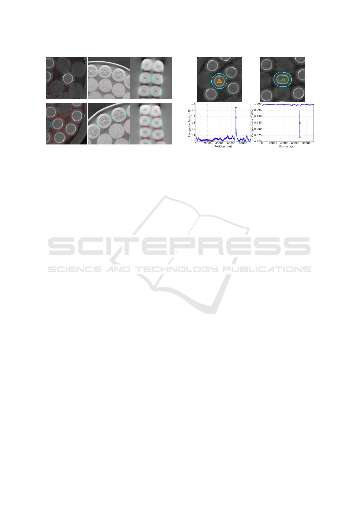
N22 (96.42%) mgb2_133 (98.22%) 18PITN01 (95.46%)

N05 (95%) mgb2_113 (97.78%) 40RRPR01 (93.4%)

Figure 8: Accuracy of the segmentation procedures on the

contours strands and the conduit (if available). For each

type of cable, we select the 2D images from the obtained

segmentations and the manual ones with the same position

along the z-axis, having the mean largest (top row) and

smallest (bottom row) DC. Both images are combined to

show false negatives (red) and false positives (cyan), su-

perimposed on the corresponding source image. For each

image, the average DC is provided between parentheses.

other types of cables, the worst error is reached for

Rutherford cables. Nevertheless, all metrics globally

show that the structures of interest (especially the con-

duit) are well segmented with, for instance, a mean

DC greater than 94% and a mean RMSD always less

than 3 pixels. The position of centerlines is also well

preserved with a mean CD always less than 1.4 pixels.

A subset of these results is illustrated in Fig. 8. For

each type of cable, we provide the 2D images from

the obtained segmentations and the manual ones with

the same position along the z-axis (where manual seg-

mentations are available) having the largest (top row)

and the smallest (bottom row) average DC. Each cou-

ple of images is then combined to show false nega-

tives (red) / false positives (cyan), superimposed on

the source image.

5.1.2 Damage Indicators

To validate the capacity of the strand sections com-

pression indicators (see Section 4.1) to detect non-

circularities, we propose the following experiment

(see Fig. 9). Two distinct locations have been iden-

tiﬁed along the same strand of the N25 cable, where

the section is either ellipsoid or circular. It has been

veriﬁed that the compression is unique along the

strand. The contours of these sections superimposed

on source images are shown on top row. On the bot-

tom row are shown the response returned by the indi-

cators along the cable. Both EF and CMPN depict a

good robustness to noise and highlight well the com-

pression by reaching a large peak at the compressed

Figure 9: Validation of the strand section compression indi-

cators on the N25 cable. Orange and green triangles are

resp. normal and compressed locations along the same

strand. On top row, the sections contours are superimposed

on source images. Red circles are locations where partial

scans have been registered.

location and remaining close to zero or one elsewhere.

The same observations were made at other locations

and on Rutherford cables.

5.1.3 Clustering

Estimate the quality of the clustering w.r.t. ground

truths is an important issue. However, no ground

truths are currently available. Due to a large num-

ber of strands and an important number of constraints

to satisfy, their construction is indeed a difﬁcult task,

especially when the cables are very short (as here).

Since the calculus of twist-pitches requires the cables

to be clustered, we believe that obtaining reasonable,

close-to-expected values, veriﬁes the clusterings.

5.2 Results

5.2.1 Cables-in-conduit

First, we have compared the values of void fraction

obtained experimentally to nominal values. The re-

sult of these comparisons is presented in Tab. 4. In

average, the void fraction differs (in absolute value)

by 1.23% and does not exceed 2.72%. Compared to

the cable N05, it also conﬁrms that the cables N22

and N25 are more likely do develop damages due to

larger void fraction.

Similarly, experimental values of twist-pitches

have been compared to nominal values. Depending of

the length of the sample, more than one or less than

one twisting periods can be available. For the studied

cables, an exhaustive comparison to references val-

ues is possible. The result of these comparisons is

ICPRAM 2016 - International Conference on Pattern Recognition Applications and Methods

548

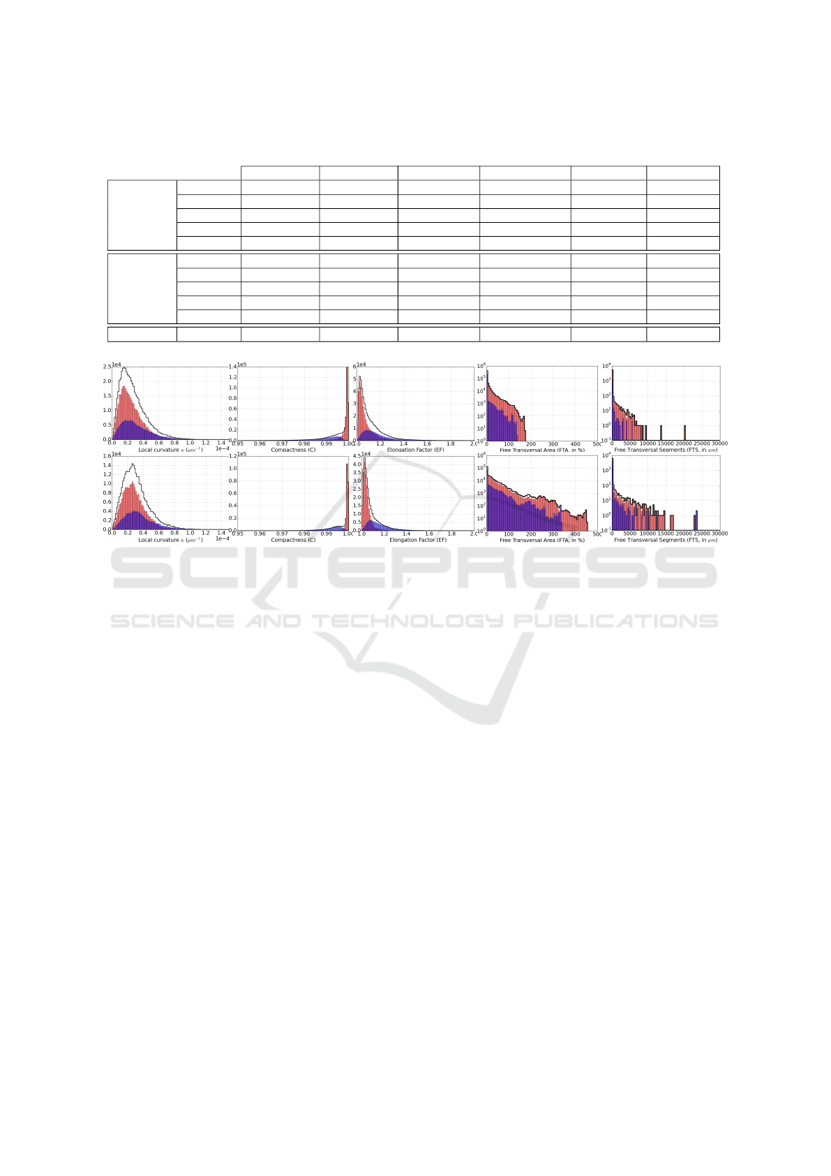
Table 3: Accuracy of the segmentation procedures with respect to ground truths for several metrics. The keyword "all" gathers

the contours of s.c. and n.s.c. strands as well as the contours of the conduit (if need be).

DC (%) VOE (%) RVD (%) RMSD (pixels) MD (pixels) CD (pixels)

In-conduit

s.c. 95.77 ±1.04 8.11 ±1.91 −7.47 ±2.17 1.60 ±0.28 3.73±0.97 0.59 ±0.36

n.s.c. 95.47 ±1.31 8.63 ±2.35 −3.04 ±2.89 1.85±0.41 5.04±1.63 1.22 ±0.84

s.c.+n.s.c. 95.63±1.18 8.35 ±2.14 −5.44 ±3.35 1.72±0.37 4.33±1.47 0.88 ±0.70

Conduit 99.67 ±0.06 0.67 ±0.12 −0.07 ±0.23 1.69±0.17 5.16±1.15 /

all 95.72 ±1.31 8.18 ±2.39 −5.33±3.41 1.71 ±0.36 4.34±1.47 /

Power

s.c. 97.86 ±0.51 4.18 ±0.97 1.06±1.69 1.62 ±0.21 4.54 ±1.03 0.86 ±0.48

n.s.c. 97.99 ±0.44 3.93 ±0.84 −0.87 ±1.53 1.57±0.23 4.27±1.02 0.83 ±0.43

s.c.+n.s.c. 97.94±0.47 4.03 ±0.90 −0.11 ±1.85 1.59±0.22 4.38±1.03 0.84 ±0.45

Conduit 99.80 ±0.10 0.39 ±0.20 0.38±0.22 2.10 ±0.35 7.06±3.43 /

all 97.97 ±0.52 3.97 ±1.01 −0.10±1.84 1.60 ±0.23 4.42±1.16 /

Rutherford s.c. 94.44 ±1.19 10.52 ±2.13 −0.99 ±3.10 2.45 ±0.74 6.49 ±2.56 1.39 ±1.05

(a) (b) (c) (d) (e)

Figure 10: Distributions of damage indicators for s.c. (pink), n.s.c. (blue) and both (black thick line) strands along the

cables-in-conduit N05 (top row) and N25 (bottom row). The y-axis of FTA and FTS is in log-scale.

shown in Tab. 5. In average, the twist-pitches dif-

fer (in absolute value) by 2.93mm (3.25%) and do

not exceed 9.38mm (7.5%). Despite the randomness

injected in these cables, this result demonstrates that

twist-pitches remain close to nominal values.

Additionally, we have computed the correlations

between local curvature and strand sections compres-

sion indicators. Then, we have decided to retain the

most relevant couples of indicators for which the ab-

solute value of the correlation coefﬁcient is larger than

0.8. Not surprisingly, EF and CMPN are well cor-

related. But most importantly, no correlation have

been identiﬁed between locally elevated curvature and

other indicators, meaning that bendings and compres-

sions locations do not coincide.

Moreover, we have compared in Fig. 10 the distri-

butions of several damage indicators (local curvature,

CMPN, EF, FTA and FTS) of two cables-in-conduit

that present different lengths, void fractions and twist-

pitches: N05 (top row) and N25 (bottom row). The

distribution of FTS is obtained by thresholding FTA at

15%, which appears to be a good value to keep signif-

icant transversal moves. For each image, we provide

both the distribution over s.c. (pink), n.s.c. (blue) and

both (black thick line) strands. For both cables, local

curvatures remain very small due to the near linearity

of strands. Also, the shape of the related distribution

suggests that it is centered around the curvature in-

duced by the twist-pitch and that local curvature max-

ima correspond to locations of potential conductivity

loss. The mean of these distributions is nearly the

same (2 ×10

−5

µm

−1

) corresponding to a curvature

radius of 50mm. Nevertheless, the mean is slightly

larger for the N25 cable. This is consistent with the

fact that this cable has smaller twist-pitch values. Ad-

ditionally, the distribution of EF and CMPN on both

cables is centered, as expected, on a value close to

one, meaning that strands sections are mainly circular.

The higher peak and longer tail of the EF distribution

on s.c. strands for N05 than for N25 indicates more

frequent and more heavily compressed strands. This

is expected as a consequence of stronger compaction

of the N05 cable.

Finally, the tail of the FTA and FTS distributions

of the N05 cable is shorter than for the N25 cable.

This means that the strands of the N05 cable have

much less space to move and that the segments where

they can move are shorter. These distributions tend

to decrease, meaning that a large area where a strand

can move is less likely to occur in the cable than a

Geometry Analysis of Superconducting Cables for the Optimization of Global Performances

549

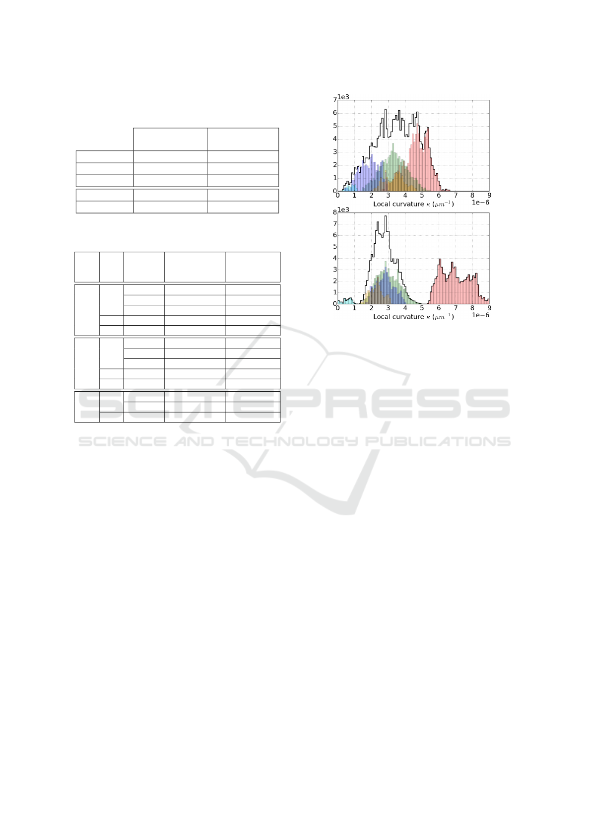
Table 4: Comparison of experimental and nominal values

of void fraction for all cables-in-conduit (top) and all power

cables (bottom).

Measured void

fraction (%)

Nominal void

fraction (%)

N05 24.16 ±0.19 25%

N22 30.28 ±0.16 33%

N25 33.13 ±0.14 33%

mgb2_113 27.57 ±0.38 24.7%

mgb2_133 27.09 ±0.41 24.7%

Table 5: Comparison of experimental and nominal values

of twist-pitches for all cables-in-conduit.

Cable Stage

Twisting

Period

Experimental

twist-pitches

(mm)

Nominal

twist-pitches

(mm)

N05

1 43.81 ±1.46 45

2 87.95 ±2.52 90

3 131.57 ±5.89 135

1 83.10 ±6.00 85

1 129.06 ±0.00 125

N22

1 43.92 ±1.26 45

2 87.82 ±2.24 90

3 131.77 ±3.63 135

1 82.22 ±2.80 85

1 115.62 ±0.00 125

N25

1 35.84 ±1.13 35

2 72.93 ±2.48 70

1 61.89 ±1.49 65

small one. Again, this is an expected consequence of

the stronger compaction of the N05 cable. Moreover,

large areas are more likely to occur for s.c. strands

than for n.s.c. strands. This is consistent with the fact

that the number s.c. strands is greater than the number

of n.s.c. strands (see Table 1).

5.2.2 Power Cables

As for cables-in-conduit, the values of void fraction

obtained experimentally from segmentations have

been ﬁrst compared to nominal values. The result of

these comparisons is available in Tab. 4. In average,

the void fraction differs (in absolute value) by 2.6%

from the nominal values and does not exceed 2.87%

(which appears to be slightly larger than for cables-

in-conduit).

Finally, we have compared in Fig. 11 the distribu-

tions of the local curvature of the two power cables:

mgb2_113 and mgb2_133. As for cables-in-conduit,

the strands have near linear trajectories, thus leading

to small values of local curvature up to 9×10

−6

µm

−1

This corresponds to a maximum radius of curvature

of 111mm. Unlike cables-in-conduit, the shape of the

related distributions is multimodal where each mode

Figure 11: Distributions of the local curvature κ along the

power cables mgb2_113 (top) and mgb2_133 (bottom) for

s.c. strands (pink), n.s.c. strands (green, blue, orange, cyan,

resp. from outer to inner stages) and all strands (black thick

line).

is centered on the local curvature of the correspond-

ing concentric layer of strands. Each mode appears to

be well separated from the others. Whereas we expect

to get an increasing local curvature as the concentric

layer becomes large, it seems to be only partially true.

A possible explanation is the existence of slightly dif-

ferent twist-pitches among these layers.

5.2.3 Rutherford Cables

In Fig. 12, we have compared the distributions of

several damage indicators (local curvature, CMPN

and EF) of two Rutherford cables presenting a dif-

ferent length and number of strands: 18RRPN01 and

40RRPR02. Notice that the y-axis of all images is in

log-scale to ease the analysis of results. In contrast to

the other types of cables studied, the local curvature

appears to be much larger (due to the folding of the

cable), up to 2.75 ×10

−4

µm

−1

. This corresponds to

a radius of curvature of 3.63mm. Moreover, the dis-

tribution of all indicators share the same shape. More

precisely, the head of these distributions corresponds

to the circular and straight strands with null values of

local curvature and values close to one for the other

indicators. The tail of these distributions corresponds

to compressed and curved strands, on the sides of the

cable.

Finally, the correlations between all the above in-

dicators have been computed. The most relevant cou-

ICPRAM 2016 - International Conference on Pattern Recognition Applications and Methods

550

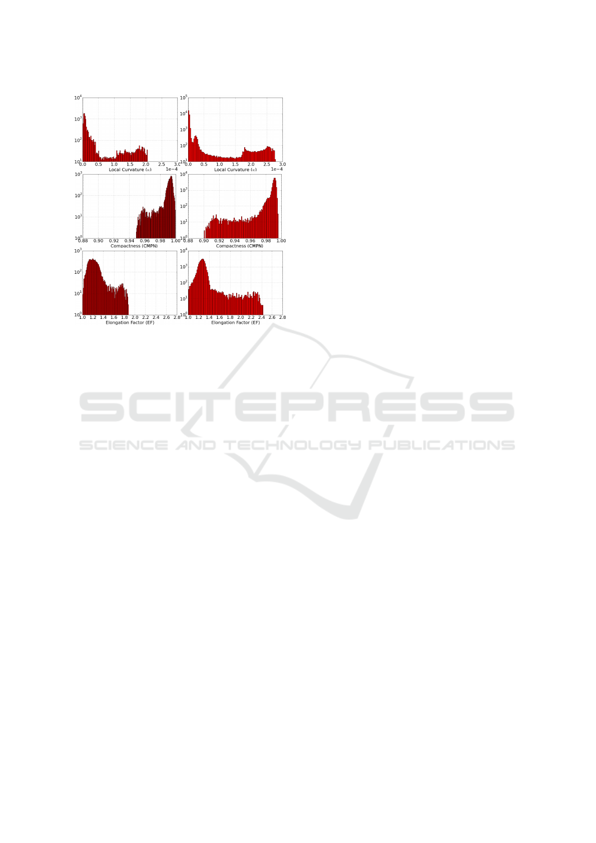
Figure 12: Distributions of the local curvature (top row),

CMPN (middle row) and the elongation factor (bottom row)

along the Rutherford cables 18RRPN01 and 40RRPR02.

For the purpose of visualization, the y-axis of all images

is in log-scale.

ples of indicators were selected as those having an ab-

solute correlation coefﬁcient above 0.8. These corre-

lations have permitted to conclude that EF and CMPN

are the most correlated ones. The obtained corre-

lations between local curvature and strand sections

compression indicators also conﬁrmed that bendings

and compressions locations coincide quite well with

a coefﬁcient of about 0.7 in absolute value.

6 CONCLUSION

This paper presents a segmentation and geometry

analysis of three types of cables and is, to our knowl-

edge, the ﬁrst one to provide methods and results to

this aim. The segmentation results exhibit a good ac-

curacy w.r.t. manually provided ground truth. The

features appear to be relevant for detecting deforma-

tions such as crushing or bending. The results are now

going to be analyzed. We have found, for instance,

that s.c. and n.s.c. strands exhibit different distribu-

tions of the crushing-related features. Similarly, no

spatial correlation between crushing and bending was

found. A further statistical analysis of the results will

be done in the future.

REFERENCES

Dice, L. (1945). Measures of the amount of ecologic asso-

ciation between species. 26(3):297–302.

Ginneken, B., Heimann, T., and Styner, M. (2007). 3D seg-

mentation in the clinic: A grand challenge.

IEC (2004). Âmes des câbles isolés. IEC Central Ofﬁce

Geneva Switzerland. CEI 60228:2004.

Ikonen, L. (2005). Pixel queue algorithm for geodesic dis-

tance transforms. 3429:228–239.

Manil, P., Mouzouri, M., and Nunio, F. (2012). Mechanical

modeling of low temperature superconducting cables

at the strand level. 22(3).

Meyer, F. (1991). Un algorithme optimal de ligne de partage

des eaux. volume 2, pages 847–859.

Milanese, A., Devaux, M., Durante, M., Manil, P., Perez, J.,

Rifﬂet, J., De Rijk, G., and Rondeaux, F. (2012). De-

sign of the EuCARD high ﬁeld model dipole magnet

FRESCA2. 22(3).

Mittelmann, H. (2007). Recent benchmarks of optimization

software.

Montero, R. (2009). State of the art of compactness and

circularity measures. 4(27):1305–1335.

Oberli, L. (2013). Development of the Nb

Sn Ruther-

ford cable for the EuCARD high ﬁeld dipole magnet

FRESCA2. 23(3).

Seidel, M. and Sturge, D. (2009). Tensile surface and struc-

ture: A pratical guide to cable and membrane con-

struction. Wiley.

Sternberg, R. (1986). Grayscale morphology. 35(3):333–

355.

Torre, A., Bajas, H., and Ciazynski, D. (2014). Mechani-

cal and electrical modeling of strands in two ITER CS

cable designs. 24(3).

Žuni

c, J. (2012). Shape descriptors for image analysis.

15(23):5–38.

Weiss, K., Heller, R., Fietz, W., Duchateau, J., Dolgetta, N.,

and Vostner, A. (2007). Systematic approach to ex-

amine the strain effect on the critical current of Nb

cable-in-conduit-conductors. 17(2):1469–1472.

Geometry Analysis of Superconducting Cables for the Optimization of Global Performances

551