Hessian Eigenfunctions for Triangular Mesh Parameterization

Daniel Mejia, Oscar Ruiz-Salguero and Carlos A. Cadavid

Laboratorio de CAD CAM CAE, Universidad EAFIT, Cra 49 No-7 Sur-50, 050022, Medellin, Colombia

Keywords:

Applied Differential Geometry, Dimensionality Reduction, Hessian Locally Linear Embedding, Manifold

Learning, Mesh Parameterization.

Abstract:

Hessian Locally Linear Embedding (HLLE) is an algorithm that computes the nullspace of a Hessian func-

tional H for Dimensionality Reduction (DR) of a sampled manifold M. This article presents a variation of

classic HLLE for parameterization of 3D triangular meshes. Contrary to classic HLLE which estimates local

Hessian nullspaces, the proposed approach follows intuitive ideas from Differential Geometry where the local

Hessian is estimated by quadratic interpolation and a partition of unity is used to join all neighborhoods. In

addition, local average triangle normals are used to estimate the tangent plane T

M at x ∈ M instead of PCA,

resulting in local parameterizations which reﬂect better the geometry of the surface and perform better when

the mesh presents sharp features. A high frequency dataset (Brain) is used to test our algorithm resulting in a

higher rate of success (96.63%) compared to classic HLLE (76.4%).

1 INTRODUCTION

Dimensionality Reduction (DR) takes a d-manifold

M ⊂ R

and computes a map h : M → R

such that: 1)

h is bijective and 2) h and h

−1

are continuous. There-

fore, h is an homeomorphism and the image of M un-

der h is a DR of M.

Mesh Parameterization can be seen as a particular

case of DR where M ⊂ R

is a triangular mesh of a

2-manifold (i.e. D = 3 and d = 2). Triangular meshes

are very common data structures in CAD CAM CAE

applications and parameterization of such meshes is

relevant for areas such as: reverse engineering, tool

path planning, feature detection, etc.

A natural way to handle Mesh Parameterization is

to attack the problem from the point of view of DR.

Classic HLLE (Hessian Locally Linear Embedding)

(Donoho and Grimes, 2003) is an algorithm which

proposes to compute a DR of M by computing the

eigenvectors of a Hessian functional. This article pro-

poses a modiﬁcation for the classic HLLE which can

be applied to triangular meshes. Our proposed ap-

proach computes a partition of unity on M and esti-

mates the tangent Hessian on each neighborhood N

M by interpolating any function f with second degree

polynomials. In addition, local average triangle nor-

mals are used to compute the tangent local plane T

of M which is more consistent than Principal Compo-

nent Analysis (PCA) specially for surfaces with sharp

features.

The remainder of this article is organized as fol-

lows: Section 2 reviews the relevant literature. Sec-

tion 3 describes the implemented methodology. Sec-

tion 4 discusses and compares the results of the pro-

posed approach against classic HLLE. Section 5 con-

cludes the paper and introduces what remains for fu-

ture work.

2 LITERATURE REVIEW

Given a set of points X = [x

,...,x

] ⊂ R

ly-

ing on a d-manifold M, DR seeks a homeomorphic

function h : M → R

such that the set of points

[h(x

),h(x

),...,h(x

)] ⊂ R

compose a DR of X.

For the rest of the article we assume D = 3 and d = 2,

turning the DR problem into a Mesh Parameterization

one.

The most popular algorithm for DR is the Princi-

pal Component Analysis (PCA). PCA is a linear al-

gorithm which parameterizes M by projecting X onto

a plane, which is only a valid parameterization if h is

linear. However, this assumption limits the algorithm

making it useful only for trivial cases.

For nonlinear manifolds, other approaches have

been proposed in the literature. For example, Isomap

(Tenenbaum et al., 2000) attempts to compute an

isometric parameterization of M by computing the

geodesic distances in M and reproducing them in the

Mejia, D., Ruiz-Salguero, O. and Cadavid, C.

Hessian Eigenfunctions for Triangular Mesh Parameterization.

DOI: 10.5220/0005668200730080

In Proceedings of the 11th Joint Conference on Computer Vision, Imaging and Computer Graphics Theory and Applications (VISIGRAPP 2016) - Volume 1: GRAPP, pages 75-82

ISBN: 978-989-758-175-5

parameter space. Isomap has been succesfully ap-

plied in the context of Mesh Parameterization (Sun

and Hancock, 2008; Ruiz et al., 2015). Usually a

shortest path algorithm such as Dijktra’s or Floyd’s

is used to estimate geodesic distances which fail for

non-convex manifolds such as surfaces with holes.

Spectral theory is an important branch of graph

theory where several DR algorithms have been de-

rived. Laplacian Eigenmaps (Belkin and Niyogi,

2003) computes the Laplacian matrix which acts over

any function deﬁned on the graph of M measur-

ing its curvature. Diffusion Maps (DM) (Lafon and

Lee, 2006) computes the Markov matrix which esti-

mates the transition probability between vertices of

the graph of M. DR is achieved in both cases by com-

puting the eigenvectors of these matrices respectively.

Spectral algorithms preserve topologic properties of

the underlying graph keeping adjacent points near in

the parameter space. However, these algorithms usu-

ally fail to preserve geometric properties which be-

comes important in Mesh Parameterization applica-

tions.

Other DR algorithms focus on a more local ap-

proach where each neighborhood is ﬁrst parame-

terized locally and then all the neighborhoods are

aligned in the parameter space trying to preserve ge-

ometric properties. Locally Linear Embedding (LLE)

(Roweis and Saul, 2000) expresses each point in M

as a linear combination of its neighborhs and then

computes the DR attempting to preserve such struc-

ture in the parameter space for all the points. Simi-

larly, Local Tangent Space Alignment (LTSA) (Zhang

and Zha, 2002) projects each neighborhood onto the

tangent plane via PCA and then attempts to align

all the neighborhoods in the parameter space using

rigid transformations. These algorithms highly pre-

serve geometric properties and perform well for non-

convex manifolds. However, they expect that each

neighborhood lies on a linear subspace which fails at

sharp features of 3D meshes resulting in non-bijective

parameterizations. Most Mesh Parameterization al-

gorithms also follow this idea by aligning triangles in

the parameter space preserving geometric properties

for each triangle (L

evy et al., 2002; Liu et al., 2008;

Athanasiadis et al., 2013; Smith and Schaefer, 2015)

or as LLE does, by locally convex linear combinations

(Floater, 1997; Lee et al., 2002). Other Mesh Param-

eterization algorithms compute the resulting parame-

terization in terms of the angles of the Mesh (Sheffer

and de Sturler, 2001; Kharevych et al., 2006; Zayer

et al., 2007).

2.1 Classic Hessian Locally Linear

Embedding (HLLE)

Classic Hessian Locally Linear Embedding (Donoho

and Grimes, 2003) is a DR algorithm which com-

bines ideas from LLE and LTSA with ideas from di-

crete differential geometry. HLLE computes a local

parameterization of each neighborhood using PCA.

But instead of aligning all neighborhoods by a rigid

mapping, HLLE estimates a Hessian functional H on

M (similar to Laplacian Eigenmaps which estimates a

Laplacian functional) and computes the DR of M by

estimating the kernel of H , i.e. ker(H ) = { f |H f =

0}.

In order to compute H , the tangent Hessian H

tan

must be deﬁned (Donoho and Grimes, 2003):

tan

f =





∂

∂b

∂

∂b

∂

∂b

∂

∂b





, (1)

where b

∈ R

is an orthonormal basis for the

tangent plane T

M at x. If f = { f

, f

,..., f

} with

= f (x

) is the function f restricted to the set of

points X, then the Hessian functional H is deﬁned

as (Donoho and Grimes, 2003):

H f =

tan

f k

dA =

∑

i=1

tan

f k

≈ f

Kf (2)

where f ∈ C

(M) is a smooth function deﬁned on

M, k · k

is the Frobenius norm, dA is a surface dif-

ferential, (M

, φ

) is a partition of unity of M and

K = (K

,...,K

) is the discrete Hessian estima-

tor computed by adding each local Hessian estimator

at each neighborhood N

Since the matrix K approximates the Hessian

functional on M, the kernel of H can be estimated by

solving the following minimization problem (Donoho

and Grimes, 2003):

= arg min

Kf, h

= arg min

s.t.

k = 1, h

⊥ 1, h

⊥ h

i = 1, 2

(3)

where h

= [h

),...,h

)]

and h

),...,h

)]

are the respective coordi-

nates of X in the parameter space. The constant

function f (x) = c, c ∈ R, is in the kernel of H (the

Hessian of any constant function is 0 as per eq. (1)).

Therefore, the constraint h

⊥ 1 avoids collapsing

all the vertices to a single point. The constraint

GRAPP 2016 - International Conference on Computer Graphics Theory and Applications

⊥ h

guarantees linear independence which avoids

collapsing the surface into a line. The constraint

k = 1 ﬁxes the scale of the solution.

Eq. (3) can be solved by computing the eigenvec-

tors of K associated to the second and third lowest

eigenvalue (the eigenvector associated to the lowest

eigenvalue corresponds to the constant function 1).

Basically, classic HLLE algorithm consists of: 1)

estimate the local Hessian functionals K

...,K

and the Hessian functional K = K

+ K

+ ··· + K

and 2) compute the eigenvectors of K with the small-

est eigenvalue (Donoho and Grimes, 2003).

Like LLE and LTSA, classic HLLE may present

problems for datasets with sharp features resulting in

non-bijective mappings. In addition, the computation

of the matrix K

which estimates the local Hessian

functional H |

is not consistent with the deﬁnition in

eq. (2) as only Hessian nullspaces are computed.

Conclusions of the Literature Review. In Mesh Pa-

rameterization applications, the preservation of geo-

metric properties is a priority over topology preser-

vation. Algorithms such as Laplacian Eigenmaps

and DM present highly distorted parameterizations.

Therefore, algorithms that preserve geometric prop-

erties such as Isomap, LLE, LTSA and classic HLLE

are more effective. However, these algorithms present

drawbacks such as the inability to work with con-

vex datasets or high frequency datasets, which are

very common in engineering applications. Mesh Pa-

rameterization algorithms do not face such problems.

However they are only restricted to triangular meshes.

To partially overcome these problems, this arti-

cle proposes a variation of the classic HLLE algo-

rithm for parameterization of triangular meshes. Clas-

sic HLLE algorithm is selected for this purpose since

such algorithm has provided better experimental re-

sults for Mesh Parameterization than other DR algo-

rithms (Ruiz et al., 2015). Also, since HLLE is a DR

algorithm, the proposed approach can be easily ex-

tended to meshes composed of non-triangular faces

posing a potential advantage over traditional Mesh

Parameterization algorithms.

3 METHODOLOGY

In order to parameterize M, we propose to follow the

same idea of the classic HLLE which is described in

section 2.1 (Donoho and Grimes, 2003): 1) estimate

the tangent Hessian H

tan

and the Hessian functional

at each N

, 2) estimate the Hessian functional H on

M as per eq. (2) and 3) estimate the kernel of H for

Mesh Parameterization via eigendecomposition. The

algorithm is brieﬂy described below:

1. For each neighborhood estimate the tangent plane

M at x

by computing the local average normal

vector

and compute a local parameterization O

by projecting N

onto T

2. Estimate the tangent Hessian H

tan

f and kH

tan

f k

at x

by quadratic interpolation.

3. Apply the partition of unity φ

to estimate the local

Hessian functional

tan

dA ≈ f

4. Estimate the global Hessian functional H ≈ K =

∑

i=1

5. Compute two orthogonal functions h

and h

which solve the optimization problem posed in eq.

(3) by eigendecomposition of the matrix K.

The steps of the algorithm are detailed below.

3.1 Tangent Plane T

M and Local

Parameterization O

In order to estimate the tangent Hessian H

tan

at x

the tangent plane T

M at x

is estimated. Classic

HLLE estimates T

M applying PCA on N

. However,

we propose to estimate T

M using the information of

the triangulation T as follows: let {t

,...} and

,...} be the set of triangles adjacent to x

and

their corresponding normal vectors respectively. Set

M as the plane with origin x

and normal n

(where

is the average of {n

,...}). Finally, O

is com-

puted by projecting N

onto T

Using the local average adjacent normals to com-

pute T

M usually results in better approximations of

the tangent plane than PCA and if N

belongs to a

sharp region, PCA may fail to recover a bijective pa-

rameterization while the local average normals pa-

rameterization has a better chance of being bijec-

tive. These local parameterizations affect the result-

ing global parameterization in the sense that local

non-bijectivity results in a folding of the surface in

the global parameterization.

3.2 Tangent Hessian H

tan

f and

tan

f k

The deﬁnition of tangent Hessian in eq. (1) requires

a smooth function deﬁned on M. Quadratic inter-

polation is used in order to estimate such Hessian

in a discrete surface. Let [b

] be an orthonor-

mal basis of T

M at x

. Therefore, any point p on

M at x

can be expressed as p = ub

+ vb

+ x

Let {u

,...,u

} and {v

,...,v

} be the cor-

responding coordinates of O

in this basis. If f

Hessian Eigenfunctions for Triangular Mesh Parameterization

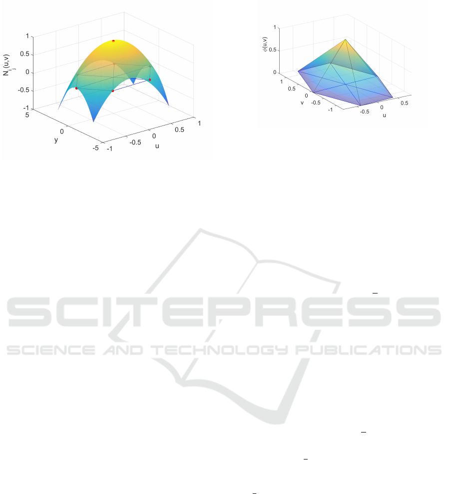
Figure 1: Quadratic interpolation function N

at N

such

that N

) = 1 if j = k, 0 otherwise.

{ f

, f

,..., f

} are the values of f restricted to N

then f can be interpolated at T

M by a second order

polynomial as follows:

f (u,v) =

∑

j=1

(u,v) f

, (4)

with N

(u,v) = α

+ β

uv + γ

+ δ

u + ε

v + ζ

Since f (u

) = f

, the interpolation functions N

are required to satisfy N

) = 1 if j = l and

) = 0 if j 6= l (ﬁg. 1). The coefﬁcients of

are computed by solving the arising linear sys-

tem of equations in a least squares sense. Afterwards,

equation (1) can be approximated as:

tan

f ≈



2α

2γ



, (5)

where α

, β

and γ

are column vectors with the cor-

responding coefﬁcients of the quadratic terms in eq.

(4). Therefore, the norm of the tangent Hessian can

be estimated as kH

tan

f k

≈ f

, where C

is a sym-

metric matrix deﬁned as:

= 4α

+ 2β

+ 4γ

(6)

3.3 Partition of Unity φ

φ and Local

Hessian Functional K

Eq. (2) requires a partition of unity (M

,φ

) deﬁned

on M. A partition of unity φ

φ =

{

,φ

,...,φ

}

is a set

of functions satisfying the following properties:

1. M

is an open subset of M.

i=1

= M.

3. φ

: M → [0,1].

4. φ

(x) = 0 if x /∈ M

Figure 2: Partition of unity φ

for a selected neighborhood

. φ

equals to 1 at x

and vanishes to 0 at adjacent points.

∑

i=1

(x) = 1 for all x ∈ M.

A partition of unity for M can be build as a set

of piecewise linear functions such that for N

, φ

deﬁned as:

) =

(

1 if i = j

0 otherwise

, ∀ j = 1,2,...,n. (7)

By its deﬁnition in eq. (7), φ

vanishes at other

neighborhoods. Therefore:

dA =

∑

, (8)

where A

is the area of the j-th adjacent triangle of

. It is not hard to check that eq. (7) satisﬁes the

properties of a partition of unity if M is a triangular

mesh.

Finally, from eqs. (6) and (8) the local Hessian

functional in eq. (2) can be estimated:

tan

f k

dA ≈





∑

. (9)

The matrix



∑



estimates the local Hes-

sian functional for any f

. Therefore, the matrix K

built as an n×n symmetric matrix which has the terms



∑



at the indices dictated by (N

), and

zeros elsewhere.

3.4 Global Hessian H and

Parameterization of M

The Hessian functional is estimated exactly as de-

scribed in (Donoho and Grimes, 2003) by adding each

local Hessian: H ≈ K =

∑

. Finally, the parame-

terization h

, h

of M is achieved by solving the min-

imization problem in eq. (3) via eigendecomposition

of the matrix K.

GRAPP 2016 - International Conference on Computer Graphics Theory and Applications

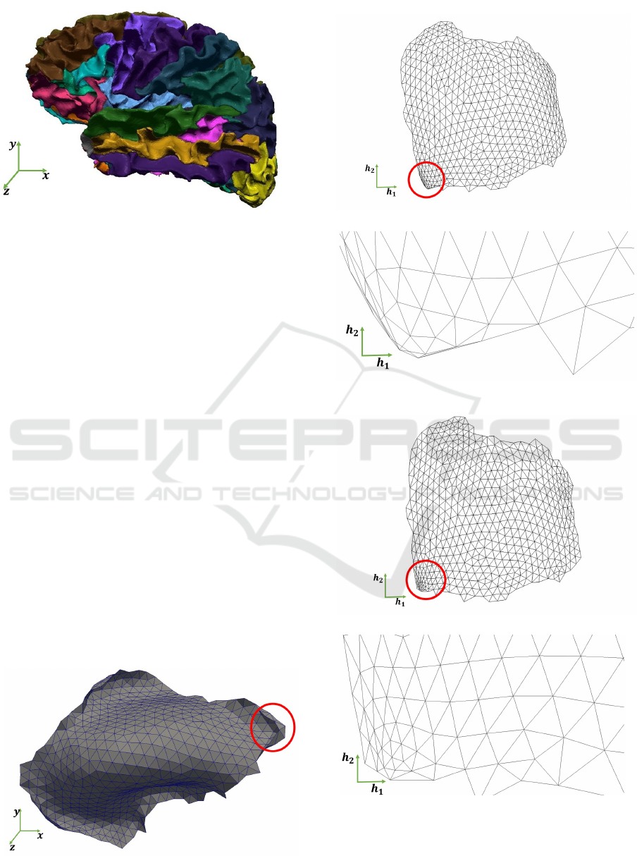
Figure 3: Segmented Brain dataset.

4 RESULTS AND DISCUSSION

In this section we present and discuss the parame-

terization results obtained for the segmented Brain

dataset (Desikan et al., 2006) and the Face dataset

(Ruiz et al., 2015). We also present an asymptotic

time complexity comparison for our algorithm and

several Mesh Parameterization algorithms.

4.1 Datasets

The Brain dataset (ﬁg. 3) presents several challenges

in terms of Mesh Parameterization given the high cur-

vatures and the low developability of the surface. We

remeshed all the sub-meshes and some of them were

also partitioned manually prior to parameterization.

From the 89 sub-meshes, classic HLLE computed

only 68 (76.40%) bijective parameterizations while

our algorithm computed 86 (96.63%) bijective map-

pings.

The Left Hemisphere - Frontal Pole sub-mesh (ﬁg.

4) presents a high frequency zone near a corner. Fig. 5

presents the parameterization results obtained by clas-

Figure 4: Left Hemisphere - Frontal Pole mesh. The red

ellipse marks a high frequency zone.

(a) Non-bijective parameterization with classic HLLE.

(b) Zoom into high frequency zone for classic HLLE (non-

bijective).

(d) Zoom into high frequency zone for our algorithm (bi-

jective).

Figure 5: Parameterization results for the Left Hemisphere

- Frontal Pole mesh. The red ellipse marks the high fre-

quency zone.

Hessian Eigenfunctions for Triangular Mesh Parameterization

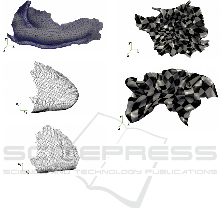
(a) Left Hemisphere - Rostral Anterior Cingulate mesh.

(b) Non-bijective parameterization with classic HLLE.

Figure 6: Parameterization results for the Left Hemisphere

- Rostral Anterior Cingulate mesh with classic HLLE and

our algorithm.

sic HLLE and our algorithm. As described in section

3.1 Classic HLLE parameterization (ﬁg. 5(a)) com-

putes local non-bijective parameterizations at such

sharp zone. As a consequence, the parameterized sur-

face folds as detailed in ﬁg. 5(b) resulting in a non-

bijective parameterization. On the other hand, our al-

gorithm does not face this problem and correctly un-

folds the surface recovering a bijective parameteriza-

tion (ﬁgs. 5(c) and 5(d)).

Fig. 6 presents the parameterization results for the

Right Hemisphere - Temporal Pole sub-mesh which

presents several sharp sections (ﬁg. 6(a)) using the

classic HLLE algorithm and our algorithm. Clas-

sic HLLE fails to adequately parameterize some lo-

cal features of the surface resulting in a non-bijective

mapping (ﬁg. 6(b)). Again, our algorithm does not

face this problem resulting in a bijective mapping (ﬁg.

6(c)). In addition, less shape distortion can be evi-

(a) Left Hemisphere - Rostral Middle Frontal texture map.

(b) Right Hemisphere - Lateral Occipital bijective texture

map.

Figure 7: Texture map of other bijective mappings from the

Brain dataset computed with our algorithm.

denced from our algorithm compared to classic HLLE

parameterization (ﬁgs. 6(b) and 6(c)) due to the ex-

plicit computation of the local Hessian functional.

Results of our algorithm for other sub-meshes of

the Brain are presented in ﬁg. 7. The texture map

of a chessboard pattern illustrates the angular distor-

tion of the respective parameterization where less lo-

cal distortion is present if the corners of the mapped

rectangles are near 90 degrees. All the four param-

eterizations are bijective despite the high frequencies

of the sub-meshes.

Highly non-developable meshes still pose a prob-

lem to our algorithm. Fig. 8 presents a case of the

Brain dataset where the algorithm fails to recover a

bijective parameterization. In this case the parameter-

ization degenerates near the boundary (i.e. triangles

overlap) in the parameter space due to the high non-

developability of such zones in the surface.

Finally, ﬁg. 9 presents the texture map (computed

by our algorithm) of a chessboard pattern onto the

Face dataset. The underlying parameterization is bi-

jective, handling easily the non-convex parts (i.e. eye

holes) with low shape distortion.

GRAPP 2016 - International Conference on Computer Graphics Theory and Applications

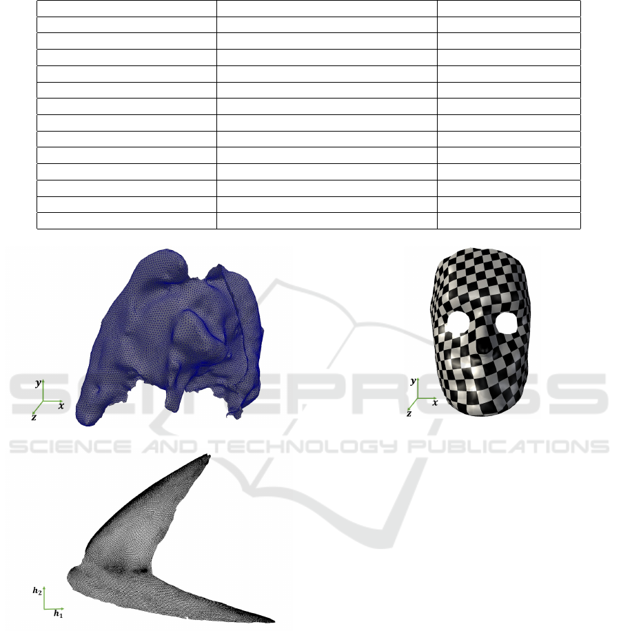
Table 1: Appraisal of time complexity of Mesh Parameterization algorithms. c denotes the number of iterations before

convergence for that particular algorithm while |∂M| denotes the number of vertices at the boundary of M.

Reference Algorithm Complexity

N/A Our algorithm O(c · n)

(Donoho and Grimes, 2003) Classic HLLE O(c · n)

(Floater, 1997) Floater Parameterization O(c · n)

(Yoshizawa et al., 2004) Stretch Minimizing Parameterization O(c

· c

· n)

(Desbrun et al., 2002) Intrinsic Parameterization O(c · n)

evy et al., 2002) LSCM O(c · n)

(Lee et al., 2002) Virtual Boundary Parameterization O(c

· n + c

· |∂M|)

(Zayer et al., 2007) LinearABF O(c · n)

(Liu et al., 2008) ASAP O(c · n)

(Liu et al., 2008) ARAP O(c

· c

· n + c

· |∂M|)

(Sheffer and de Sturler, 2001) ABF O(c

· c

· n)

(Kharevych et al., 2006) Discrete Conformal Mappings O(c

· c

· n

(Smith and Schaefer, 2015) Free Boundary Parameterization O(c · (n + |∂M|))

(a) High Frequency - High Curvature dataset.

(b) Non-bijective parameterization of the High Frequency -

High Curvature dataset with our algorithm.

Figure 8: Failure test for our algorithm.

4.2 Time Complexity Comparison

In order to compare our algorithm with other Mesh

Parameterization algorithms, table 1 presents an ap-

praisal of the time complexity of several Mesh Pa-

rameterization algorithms. Classic HLLE and our al-

gorithm compute the ﬁrst three eigenvectors of the

Hessian estimator by the Implicitly Restarted Lanczos

Figure 9: Texture map on the Face dataset computed with

our algorithm.

Method with time complexity O(c · n) (here we de-

note c ≥ 1 as the number of iterations executed by the

algorithm before convergence). Other Mesh Parame-

terization algorithms rely on solving a linear system

of equations, which is usually solved by a Conjugate

(or Bi-Conjugate) Gradient Method once (O(c · n)) or

several times (O(c

· c

· n)). It is important to note

that c is not the same between algorithms, but it is

stated that such number is relatively low in applica-

tions after matrix preconditioning as well as use of

initial parameterizations in iterative algorithms.

5 CONCLUSIONS

This article presents a variation of the classic HLLE

algorithm for parameterization of triangular meshes.

Classic HLLE was selected for this purpose since it

has shown experimentally better results than other DR

algorithms for Mesh Parameterization. An intuitive

approach from Differential Geometry is followed by

estimating locally the tangent Hessian with quadratic

Hessian Eigenfunctions for Triangular Mesh Parameterization

interpolation and computing a partition of unity for

the triangular mesh M as opposed to classic HLLE

approach. In addition, each local parameterization is

achieved by projecting onto the local average trian-

gle normals plane instead of the usual PCA, which

reﬂects better the local geometry of the surface spe-

cially in cases of sharp features.

The Brain dataset was parameterized with both

Classic HLLE and our algorithm resulting in a higher

rate of success (96.63%) for our approach against

classic HLLE (76.40%). The Face dataset was also

considered, resulting in a bijective parameterization

with low shape distortion despite having holes. Com-

plexity analysis showed that our algorithm asymptot-

ically behaves similar to Mesh Parameterization algo-

rithms that rely on solving a linear system of equa-

tions only once.

5.1 Ongoing Work

Segmentation of complex meshes with high gaus-

sian curvatures into smaller ones increases the prob-

ability of ﬁnding bijective parameterizations. There-

fore, automatic mesh segmentation for this task be-

comes crucial for parameterization of large and com-

plex datasets.

ACKNOWLEDGEMENTS

This research has been funded by the Research Group

and College of Engineering at Universidad EAFIT,

Colombia.

REFERENCES

Athanasiadis, T., Zioupos, G., and Fudos, I. (2013).

Efﬁcient computation of constrained parameteriza-

tions on parallel platforms. Computers & Graphics,

37(6):596–607. Shape Modeling International (SMI)

Conference 2013.

Belkin, M. and Niyogi, P. (2003). Laplacian eigenmaps

for dimensionality reduction and data representation.

Neural Computation, 15(6):1373–1396.

Desbrun, M., Meyer, M., and Alliez, P. (2002). Intrinsic pa-

rameterizations of surface meshes. Computer Graph-

ics Forum, 21(3):209–218.

Desikan, R. S., S

egonne, F., Fischl, B., Quinn, B. T., B,

C. D., Blacker, D., Buckner, R. L., Dale, A. M.,

Maguire, R. P., Hyman, B. T., Albert, M. S., and Kil-

liany, R. J. (2006). An automated labeling system

for subdividing the human cerebral cortex on +mri

scans into gyral based regions of interest. NeuroIm-

age, 31(3):968–980.

Donoho, D. L. and Grimes, C. (2003). Hessian eigen-

maps: Locally linear embedding techniques for high-

dimensional data. Proceedings of the National

Academy of Sciences, 100(10):5591–5596.

Floater, M. S. (1997). Parametrization and smooth approxi-

mation of surface triangulations. Computer Aided Ge-

ometric Design, 14(3):231–250.

Kharevych, L., Springborn, B., and Schr

oder, P. (2006).

Discrete conformal mappings via circle patterns. ACM

Transactions on Graphics, 25(2):412–438.

Lafon, S. and Lee, A. (2006). Diffusion maps and coarse-

graining: a uniﬁed framework for dimensionality re-

duction, graph partitioning, and data set parameteriza-

tion. Pattern Analysis and Machine Intelligence, IEEE

Transactions on, 28(9):1393–1403.

Lee, Y., Kim, H. S., and Lee, S. (2002). Mesh parameteriza-

tion with a virtual boundary. Computers & Graphics,

26(5):677–686.

evy, B., Petitjean, S., Ray, N., and Maillot, J. (2002). Least

squares conformal maps for automatic texture atlas

generation. In ACM, editor, ACM SIGGRAPH con-

ference proceedings.

Liu, L., Zhang, L., Xu, Y., Gotsman, C., and Gortler, S. J.

(2008). A local/global approach to mesh parameteri-

zation. In Proceedings of the Symposium on Geometry

Processing, SGP ’08, pages 1495–1504, Aire-la-Ville,

Switzerland, Switzerland. Eurographics Association.

Roweis, S. T. and Saul, L. K. (2000). Nonlinear dimension-

ality reduction by locally linear embedding. Science,

290(5500):2323–2326.

Ruiz, O. E., Mejia, D., and Cadavid, C. A. (2015). Trian-

gular mesh parameterization with trimmed surfaces.

International Journal on Interactive Design and Man-

ufacturing (IJIDeM), pages 1–14.

Sheffer, A. and de Sturler, E. (2001). Parameterization of

faceted surfaces for meshing using angle-based ﬂat-

tening. Engineering with Computers, 17(3):326–337.

Smith, J. and Schaefer, S. (2015). Bijective parameteri-

zation with free boundaries. ACM Transactions on

Graphics, 34(4):70:1–70:9.

Sun, X. and Hancock, E. R. (2008). Quasi-isometric param-

eterization for texture mapping. Pattern Recognition,

41(5):1732–1743.

Tenenbaum, J. B., de Silva, V., and Langford, J. C. (2000).

A global geometric framework for nonlinear dimen-

sionality reduction. Science, 290(5500):2319–2323.

Yoshizawa, S., Belyaev, A., and Seidel, H.-P. (2004). A

fast and simple stretch-minimizing mesh parameteri-

zation. In Shape Modeling Applications, 2004. Pro-

ceedings, pages 200–208.

Zayer, R., L

evy, B., and Seidel, H.-P. (2007). Linear angle

based parameterization. In ACM/EG Symposium on

Geometry Processing conference proceedings.

Zhang, Z. and Zha, H. (2002). Principal manifolds and

nonlinear dimension reduction via local tangent space

alignment. SIAM Journal of Scientiﬁc Computing,

26:313–338.

GRAPP 2016 - International Conference on Computer Graphics Theory and Applications