Efﬁcient Culling Techniques for Interactive Deformable NURBS

Surfaces on GPU

Raquel Concheiro

, Margarita Amor

, Emilio J. Padr

and Michael Doggett

Computer Architecture Group, Universidade da Coru

na, A Coru

na, Spain

Lund University Graphics Group, Lund University, Lund, Sweden

Keywords:

NURBS, Real-time and Interactive Methods, Culling Techniques, Deformable Surfaces.

Abstract:

NURBS (Non-uniform rational B-splines) surfaces are the standard freeform representation in Computer-

Aided Design (CAD) applications. Rendering NURBS surfaces accurately while they are interactively manip-

ulated and deformed is a challenging task. In order to achieve it, the elimination from pipeline in early stages

of back-facing surfaces or surface pieces is a key advantage. Furthermore, an effective interactive manipula-

tion implies that all the culling computations should be performed for each frame, facing the possibility of fast

changes in occlusion information. In this paper, different interactive culling strategies for NURBS surfaces

are presented and analyzed. These culling techniques are based on the exploitation of the geometric properties

presented in a NURBS surface, that allow easily to ﬁnd bounds for it in screen space for each frame. Further-

more, the culling overhead for our proposals is small compared to the computational saving, outperforming a

proposal without culling. An implementation of these strategies using current GPUs is presented, achieving

real-time and interactive rendering rates of complex parametric models.

1 INTRODUCTION

NURBS (Non-uniform rational B-splines) surfaces

(Piegl and Tiller, 1997) are widely employed in

CAD/CAM tools and graphics applications since their

essential features and qualities makes them an opti-

mal solution for modeling complex geometries. Even

though modern GPUs have introduced dedicated

hardware tessellation units (Sch

afer et al., 2014),

these units do not always guarantee to have enough

tessellation level or ﬂexibility to render a NURBS sur-

face with no artifacts, such as cracks, holes or creases.

Furthermore, NURBS surfaces introduce consider-

able advantages to the on-the-ﬂy shape manipulation

of highly detailed geometry, as only a few patch con-

trol points (Smith and Schaefer, 2015) need to be han-

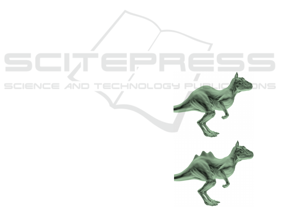
dled (see Figure 1). Clearly, adaptive rendering meth-

ods to avoid the rendering of hidden surfaces or pieces

of surfaces are key for performance. Thus, imple-

menting effective and efﬁcient culling techniques in

the rendering pipeline is deﬁnitely important.

Traditionally, there have been two main ap-

proaches to render NURBS surfaces on GPU. The

ﬁrst alternative is based on the conversion on CPU

of NURBS surfaces to other representations, such

as Catmull-Clark subdivision surfaces (Shen et al.,

Figure 1: Shape manipulation of a NURBS surface

(Killeroo Model) by interactively moving a few control

points.

2014) or B

ezier patches (Cohen et al., 1980), that can

be efﬁciently rendered on GPU (Guthe et al., 2005;

Concheiro et al., 2010; Yeo et al., 2012; Claux et al.,

Concheiro, R., Amor, M., Padrón, E. and Doggett, M.

Efﬁcient Culling Techniques for Interactive Deformable NURBS Surfaces on GPU.

DOI: 10.5220/0005677200150025

In Proceedings of the 11th Joint Conference on Computer Vision, Imaging and Computer Graphics Theory and Applications (VISIGRAPP 2016) - Volume 1: GRAPP, pages 17-27

ISBN: 978-989-758-175-5

2014; Nießner et al., 2012). The main disadvantage of

these proposals is that they can not handle deforming

NURBS surfaces interactively, since costly NURBS

surface to other representation conversions should be

performed multiple times per frame as the surface is

being deformed.

The other approach is based on rendering the

NURBS surfaces directly on GPU, with no previ-

ous conversion (Krishnamurthy et al., 2007; Krishna-

murthy et al., 2009; Concheiro et al., 2014). In (Kr-

ishnamurthy et al., 2007) and (Krishnamurthy et al.,

2009), a previous tessellation is performed on the

CPU, that creates a set of grids indicating the surface

evaluation points for different levels of detail, and

these data are sent to the GPU and stored as textures.

In (Concheiro et al., 2014), a solution for the direct

rendering of NURBS surfaces on the GPU without

any previous decomposition or tessellation to B

ezier

surfaces is presented. This proposal, called RPNS

(Rendering Pipeline for NURBS Surfaces) is based on

a primitive, KSQuad, which uses a regular and ﬂexi-

ble processing of NURBS surfaces, while maintaining

their main geometric properties to achieve real-time

rendering.

Culling is the process of removing those portions

of the scene that do not contribute to the ﬁnal render-

ing. The advantage of culling in the early stages of

the rendering pipeline is that entire objects that are

invisible can be removed, saving a great deal of com-

putation in the rest of the pipeline. When dealing

with polygons, one of the most traditional and stan-

dard culling techniques is Backface culling (Akenine-

oller et al., 2008), based on removing those poly-

gons which are invisible from the viewpoint as early

as possible.

Backpatch culling (Kumar et al., 1996) is an ex-

tension of backface culling to parametric surfaces,

based on removing these invisible patches as early as

possible. Although backpatch culling is not a novel

idea, up to now it has only been applied to B

ezier

patches. There are basically two different groups of

proposals to compute backpatch culling: based on the

popular cone-of-normals approach (Munkberg et al.,

2010; Sederberg and Meyers, 1988; Shirman and

Abi-Ezzi, 1993) and based on the use of bounding

boxes (Kumar et al., 1996; Loop et al., 2011). In

the ﬁrst group, (Sederberg and Meyers, 1988) pro-

poses a cone-of-normals derived from tangent and bi-

tangent patches, whose main drawback is the coarse

bounds that are obtained. (Shirman and Abi-Ezzi,

1993) presents a preprocessing step to compute a nor-

mal patch for a given B

ezier patch and to compute its

bounding cone-of-normals. Next, a simple test is used

to compute the culling on the ﬂy. The main drawback

of this approach is that dynamic models are not ren-

dered in real time owing to the high computational

cost. (Munkberg et al., 2010) is focused on ﬁtting this

algorithm into modern GPUs, which in turn means an

approximation in the computation of the tangent and

bi-tangent cone. With respect to the proposal based on

the computation of the bounding box of the patches,

(Kumar et al., 1996) computes the bounding box of

the normalized vectors of the normal patch, whereas

(Loop et al., 2011) constructs the B

ezier convex hull

of the parametric tangent plane. Instead of following

a backpatch culling approach, in (Nießner and Loop,

2012) an occlusion culling of patches is considered.

In contrast to previous alternatives, we present an

alternative solution for culling in the context of real-

time NURBS rendering with the RPNS proposal. Our

approach is based on the use of the KSQuad primitive,

and takes advantage of its strong convex hull prop-

erty. This makes it possible to support real-time an-

imated and deformed models and do not require any

pre-computed scene data structure. Furthermore, as

shown in the next sections, this culling attains an im-

portant reduction in the number of Fragment Shader

computations performed in a DirectX 11 implemen-

tation, which has a high impact on the overall perfor-

mance.

The basic concepts that support our culling pro-

posal and a brief description of RPNS are presented

in Section 2.

2 RENDERING PIPELINE FOR

NURBS SURFACES

The objective of RPNS is the efﬁcient and accu-

rate rendering of NURBS surfaces, preventing arti-

facts in the ﬁnal image such as cracks and holes,

either inside each surface or between neighbor sur-

faces. This makes it possible to exploit the paral-

lelism of the GPU to perform common operations

such as sketching on surfaces, interactive trimming

or surface-surface intersection. Figure 2 is a block

diagram of the RPNS pipeline. It consists of three

shaders: Geometry, Sampler and Rasterizer.

The input stream of the Geometry shader is a

primitive, denoted as KSQuad, that is based on the

regions deﬁned by the projection on the parametric

cell delimited by the different knot spans. This prim-

itive provides an efﬁcient and accurate evaluation of

NURBS surfaces in RPNS (processed in the Geome-

try stage, as shown in Figure 2). KSQuad needs no

pre-processing stage and intrinsically maintains the

main geometric properties of NURBS surfaces, such

as local support and strong convex hull. The exploita-

GRAPP 2016 - International Conference on Computer Graphics Theory and Applications

Geometry

KSQuad

Sampler

Rasterizer

KSDice

KSQuad

parametric space geometric space

Figure 2: Basic structure of RPNS’s pipeline.

tion of these properties enables us to improve perfor-

mance by applying acceleration algorithms, such as

the culling techniques described in Section 3.

In the Sampler shader, an adaptive sampling of

the KSQuad primitives is performed according to the

viewpoint, the geometric characteristics of the surface

and the boundary edges between surfaces. This sam-

pling process results in a set of sampled points or dice,

denoted as KSDice and which make it possible to ren-

der the surface without cracks or holes. Each KSDie

consists of a sampled point and additional informa-

tion such as the parametric size of the die and the

degree of the corresponding surface, and it does not

save any explicit connectivity information. Think in

KSDices as an artifact analogous to the idea of surfels

in the context of point rendering (Pﬁster et al., 2000).

The KSQuad discretization makes it possible to ﬁnd

an optimal rendering of the geometry of surfaces with

minimum redundancy. Thus, a suitable discretization

is obtained when it can be guaranteed that there is at

least one KSDice projected into the region of each

output pixel for orthographic projection. Therefore,

the objective is to reduce the number of positions to

be evaluated for each KSQuad primitive while keep-

ing the quality of the resulting image.

A NURBS surface is obtained as the tensor prod-

uct of two NURBS curves, parametric curves that are

deﬁned by its degree, a set of weighted control points,

and a knot vector. Thus, using two independent pa-

rameters u and v, the NURBS surface of degree (p,q),

respectively in both parametric directions, is given by

the equation:

S(u,v) =

∑

i=0

∑

j=0

i,p

(u) N

j,q

(v) w

i, j

∑

i=0

∑

j=0

i,p

(u) N

j,q

(v) w

i, j

, 0 ≤ u,v ≤ 1

where B

i, j

are the control points, w

i, j

are the weights,

n + 1 and m + 1 are the number of control points in

u and v parametric directions, respectively, and N

i,p

and N

j,q

are the nonrational B-spline basis function

deﬁned on two knot vectors of r = p + n + 1 and s =

q + m + 1 elements, respectively:

U =







0,··· ,0

| {z }

p+1

,··· ,x

r−p−1

,1, ···1

| {z }

p+1







V =







0,··· , 0

| {z }

q+1

,··· , y

s−q−1

,1, ···1

| {z }

q+1







The basis function N

i,p

of degree p is deﬁned for

the parametric direction u as

i,p

(u) =

u −x

i+p

−x

i,p−1

(u)+

i+p+1

−u

i+p+1

−x

i+1

i+1,p−1

(u)

(1)

with

i,0

(u) =



1 if x

≤ u < x

i+1

0 otherwise

Analogously, the basis function N

j,p

of degree q is

deﬁned for the parametric direction v.

A NURBS surface can be seen as a grid of cells

in parametric space delimited by the different knot

spans, with each cell containing a part of the sur-

face computed with the non-zero basis functions in

that interval. Knot Span Quad (KSQuad), repre-

sents a half-open interval of the parametric domain,

i+1

)×[y

j+1

), with non-zero length, and main-

tains the information of q ×p neighboring knot spans,

allowing an efﬁcient evaluation of the NURBS sur-

face in this interval. So, a KSQuad

i, j

of degree q and

p is deﬁned like

KSQuad

i, j

= {

knot span

z }| {

i+1

j+1

, B

i−p, j−q

,··· , B

i, j

| {z }

control points

weights

z }| {

i−p, j−q

,··· , w

i, j

}

being x

6= x

i+1

and y

6= y

j+1

Each KSQuad

i, j

controls a subset of the paramet-

ric domain, deﬁned by the rectangle parametric sub-

domain with corners (x

),k ∈ {i,i + 1},l ∈ {j, j +

1}, as illustrated in Figure 3. This sub-domain is

sampled into KSDice (samples) that provide a quality

render with no holes, yet increasing the performance.

Pixel accurate rendering (Yeo et al., 2012), in RPNS

proposal is determined by the level of samples for a

Efﬁcient Culling Techniques for Interactive Deformable NURBS Surfaces on GPU

Parametric Space

Model Space

, y

j+1

)

i+1

, y

j+1

)

, y

)

i+1

, y

)

S(x

, y

j+1

)

S(x

i+1

, y

j+1

)

S(x

, y

)

S(x

i+1

, y

)

Figure 3: KSQuad primitive deﬁned by a knot interval.

given KSQuad. In screen-spacel pixel coordinates,

the samples guarantees a KSDie, by at most µ pixels:

dist(p(S(x

)) − p(S(x

k+1

))) < µ,

) ≤ (x

) < (x

i+1

j+1

)

) < (x

k+1

) ≤ (x

i+1

j+1

)

(2)

where p() means a screen space projection. For in-

stance, µ = 1 implies by at most half a pixel.

3 CULLING TECHNIQUES

One beneﬁcial side effect of bringing forward the ge-

ometry stage prior to the sampling is that we can im-

prove the performance by also moving forward the

application of other techniques in the pipeline, such

as culling. Whereas backface culling is usually per-

formed after a tessellation step, we follow recent pro-

posals (Hasselgren et al., 2009) which cull before tes-

sellation to reduce as soon as possible the number of

primitives to be processed. We have called BackPatch

culling to this strategy, based on the original back-

patch idea for B

ezier from (Kumar et al., 1996), but

now applied to NURBS by means of the KSQUAD ar-

tifact. Two different early culling proposals based on

that idea are introduced in RPNS, performing culling

before the discretization stage.

A culling algorithm generates what is called the

potentially visible set (PVS), which is a prediction or

estimation of the exact visible set (EVS) (Akenine-

oller et al., 2008). A PVS is conservative if it fully

includes the EVS, so that only invisible geometry is

discarded. Otherwise, a PVS is approximate when the

EVS is not fully included, which results in rendered

images with a certain error.

Our BackPatch culling strategy sends down a PVS

to the next stages in the pipeline, an approximate

set in one proposal and a conservative one in the

other. These solutions are compared to a more clas-

sic sample-based culling solution, that generates an

EVS and we have named BackDice culling, earlier

presented in (Concheiro et al., 2014).

These three culling proposals are based on differ-

ent approaches and placed in different pipeline stages

in RPNS. BackDice culling is carried out at the end

of the RPNS sampler stage (see Figure 2), once the

samples have already been obtained. On the other

hand, BackPatch culling must be placed at the begin-

ning of the geometry stage, the ﬁrst step in RPNS’

pipeline (see Figure 2). Therefore, BackDice culling

works at sample level (KSDice in RPNS), whereas

the two BackPatch culling proposal do at patch level

(KSQuad in RPNS).

In any case, a previous view frustum culling is ap-

plied using the NURBS’ bounding box at KSQuad

level. This culling, based on the strong convex hull

property removes all KSQuads placed outside of the

viewing cone from being considered in the following

stages.

The strong convex hull property means a NURBS

surface is contained in the convex hull of its control

points. Moreover, if (u,v) is in the parametric rect-

angle deﬁned by the knot spans [x

i+1

) ×[y

j+1

then S(u, v) is in the convex hull deﬁned by the control

points {B

i−p, j−q

,. .. ,B

i, j

3.1 BackDice Culling

BackDice Culling (DC) is the backface culling pro-

posal we have implemented in RPNS. It is based

on the render primitive sampled from a KSQuad:

KSDice. As traditional pipelines are triangle ori-

ented in the rendering stages, culling is usually com-

puted on triangle polygons. However, as RPNS is

based on the rendering of pieces of parametric sur-

faces, speciﬁcally KSDice, the DiceCulling proposal

removes those KSDice not turned to the camera as

early as possible.

The BackDice Culling test is placed at the end of

the sampler stage, after the screen-mapping procedure

GRAPP 2016 - International Conference on Computer Graphics Theory and Applications

(see Figure 2). BackDice Culling decreases the num-

ber of KSDice sent to the rasterizer, since backfaced

KSDice are culled out. However, as backface culling

computations are done in the sampler stage, in this

stage workload is slightly increased meanwhile the

rasterizer workload is reduced.

3.2 BackPatch Culling

By applying a culling technique in the ﬁrst stages of

the pipeline, the number of primitives to be processed

is dramatically reduced (Hasselgren et al., 2009). To

prove this, two culling algorithms that exploit the ver-

satility and ﬂexibility offered by the use of KSQuad

in the geometry stage have been implemented. These

culling proposals are based on the strong convex hull

property of the NURBS surfaces that is preserved in

the KSQuad primitive, and it efﬁciently avoids the

evaluation of points of knot spans which do not con-

tribute to the ﬁnal image.

Therefore, the goal of our culling proposals is to

maintain the effectiveness of a conservative solution

with much less computation, discarding KSQuads as

early as possible in the rendering pipeline to improve

overall performance for deformable surfaces. Fig-

ure 4 shows four frames of an example NURBS sur-

face deformation. In the example, some KSQuads are

fully occluded in the initial frame but visible in the

following ones. As the results depicted in Section 5

prove, our culling proposal outperforms other alter-

natives without introducing any extra data structure,

achieving an effective and efﬁcient interactive expe-

rience when an important deformation is applied to

high-detailed NURBS surfaces.

Unlike Dice Culling, designed to remove KS-

Dice, the two backpatch culling proposals for RPNS,

Lightweight BackPatch Culling (LQC) and Strong

BackPatch Culling (SQC), have been designed to cull

out KSQuads earlier in the pipeline. Both Back-

Patch Culling methods are based on the potentially

visible set (PVS) and independently applied to each

KSQuad, so different KSQuads of a NURBS can be

culled out, whereas other ones are rendered. Conse-

quently, KSQuads are culled before being evaluated

into KSDice. This means higher computation costs in

RPNS’ geometry stage, but reduces the workload in

the sampler and rasterizer stages.

As both techniques have been speciﬁcally de-

signed for NURBS surfaces, they are based on the

strong convex hull property previously described.

Hence, the normal to the plane deﬁned by the skeleton

computed for each KSQuad is used instead of com-

puting the normal to the KSQuad, dramatically reduc-

ing the culling computational workload.

The proposed Light Quad Culling algorithm culls

a KSQuad

i, j

by using this simple square:



i, j

= {S(x

), S(x

i+1

), S(x

j+1

), S(x

i+1

j+1

)}

(3)

LQC is an approximate PVS technique and al-

though a fast and efﬁcient culling computation is pro-

vided, the EVS is not fully included thus the quality

of the render is slightly decreased as will be detailed

in Section 5. 

i, j

cannot guarantee that the normal of

all surface points have the same direction.

On the other hand, the SQC algorithm culls a

KSQuad

i, j

by computing the culling for a set of p ×q

squares



k,l

i, j

= {B

i−p+k, j−q+l

, B

i−p+k+1, j−q+l

i−p+k, j−q+l+1

, B

i−p+k+1, j−q+l+1

}

(4)

with 0 ≤ k ≤ p −1 and 0 ≤ l ≤ q −1. Each square

is the convex hull polygon corresponding to the ad-

jacent control points. If any of these squares is not

culled, then the KSQuad is not culled. A KSQuad

i, j

is contained in the convex hull deﬁned by the con-

trol points {B

i−p, j−q

,··· , B

i, j

}. That is, the NURBS

surface fragment that deﬁnes the parametric subset

KSQuad

i, j

is contained by the control net fragment,

p ×q squares. If any square is oriented to the view-

point, then it is possible that any point in the surface

is frontfaced. The control polygon represents a piece-

wise bilinear approximation to the surface. This ap-

proximation is improved by applying either knot in-

sertion or degree elevation. As a general rule, the

lower the degree, the closer the surface follows its

control polygon, reaching the extreme case with p =

1, when the surface is the control polygon. SQC is

a conservative PVS technique where the EVS is fully

included, as only invisible geometries are discarded,

and a high quality images are rendered.

Figure 5 shows two different scenarios for apply-

ing our culling strategies: for a high-degree surface

(Figure 5a), there are few knots in the NURBS and the

difference between the results obtained by the approx-

imative and the conservative strategies, 

i, j

and 

k,l

i, j

is greater; however, for a low-degree surface (Fig-

ure 5b) the squares 

i, j

comes close to the actual sur-

face, so a similar PVS is obtained in both strategies,

although with an marked reduction in performance in

the approximative method (as shown in Section 5).

The introduction of these Quad Culling techniques

in RPNS results in an important reduction in the com-

putational load of the sampler and rasterizer stages,

although this is accompanied by a slight increase in

the computation of the geometry stage.

Efﬁcient Culling Techniques for Interactive Deformable NURBS Surfaces on GPU

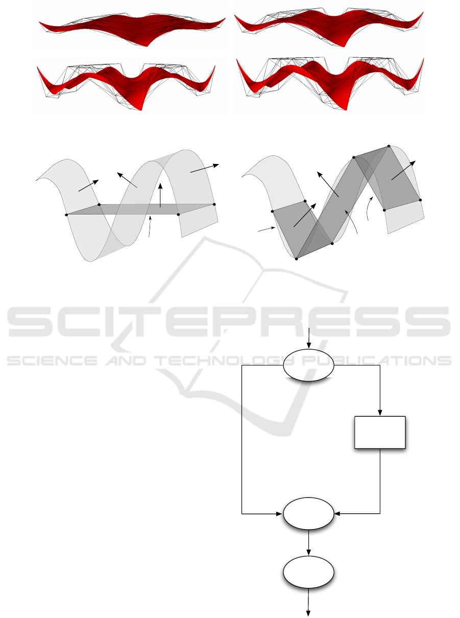
Figure 4: Example of NURBS surface deformation.

KSQuad

S(x

, y

j+1

)

S(x

, y

)

S(x

i+1

, y

j+1

)

S(x

i+1

, y

)

(a)

KSQuad

k+1

S(x

j+1

)

S(x

)

S(x

i+1

)

S(x

i+1

j+1

)

S(x

i+2

j+1

)

KSQuad

k+2

S(x

i+3

)

S(x

i+2

)

S(x

i+3

j+1

)

(b)

Figure 5: KSQuad-based culling (a) high degree NURBS (b) low degree NURBS.

4 TECHNIQUES OF CULLING

ON CURRENT GPUS USING

DIRECTX11

With DirectX11 three new stages (hull shader, tessel-

lator unit and domain shader) were introduced to sup-

port programmable tessellation (Sch

afer et al., 2014).

These stages are inserted between the vertex and the

geometry shader. The hull shader and the domain

shader are programmable stages, whereas the unit

where the real data expansion happens, the tessella-

tor, is a conﬁgurable stage. Figure 6 depicts how

a KSQuad is processed in DirectX11 according to

RPNS proposal.

Hull shader is invocated once for each input primi-

tive, KSQuad in our proposal. It is the ﬁrst stage of the

tessellation procedure and it conﬁgures tessellator and

domain shader execution. Hence, hull shader gener-

ates two different outputs to guide the tessellation pro-

cedure, one output is sent to the domain shader while

the other one is sent to the tessellator. Both outputs in-

clude the tessellation factors which are generated on-

the-ﬂy in the hull shader. In this shader a view frus-

tum culling is applied for each KSQuad. Furthermore,

LQC or SQC could be chosen to cull out KSQuad ear-

lier in the pipeline.

Domain shader receives the parametric coordi-

Hull

Shader

HS input: KSQuad

Domain

Shader

Tessellator

HS output:

if No culling

- KSQuad control points

- Tessellation factors

HS output:

- Tessellation factors

Tessellation output:

- Samples KSDice

(parametric coordinates)

Geometry

Shader

Domain output:

- KSDice

Geometry output:

if no culling

- KSDice Triangles

Figure 6: KSQuad processing in RPNS on DirectX11.

GRAPP 2016 - International Conference on Computer Graphics Theory and Applications

nates from the tessellator as well as the input prim-

itive and the tessellator factors from the hull shader.

According to the received data, these parametric co-

ordinates are evaluated in the domain shader, that is

invocated once for each parametric coordinate gen-

erated in the tessellator. The four corners of each

KSDie, S(x

), S(x

+ δ

), S(x

+ δ

), and

S(x

+ δ

), are efﬁciently evaluated in the DS

by taking advantage of access locality and avoiding

redundant computations. Let us emphasize that like

Reyes vertex shading, RPNS also allows the user to

specify an arbitrary shading rate. In Reyes, shading

rate is expressed in samples per pixel meanwhile we

specify samples per KSDie in RPNS, with a value of

4.0 in our implementation. A more efﬁcient RPNS

implementation would adaptively choose the shading

rate per KSDie, but that objective is beyond the scope

of this paper.

The output from the DS is sent to the Geometry

Shader, where two triangles are generated for each

KSDie due to the triangle-oriented graphics pipeline

of current GPUs. Furthermore, to optimize the ren-

dering of NURBS surfaces we include the evaluation

of EVS in the Geometry shader. This culling stage

has a high impact on the overall performance, since

it achieves an important reduction in the number of

KSDice to get rasterized. On the other hand, in the

Geometry Shader, the KSDie could be sampled again

in order to assure that a higher subdivision level is

applied to non-ﬂat regions. Furthermore, a bound-

ary region test detects the regions of KSDice that are

boundaries to other surfaces and applies the highest

subdivision factor to prevent cracks between adjacent

surfaces.

5 EXPERIMENTAL RESULTS

In this section we present the results obtained with

our culling methods implemented in RPNS. Our test

platform is an Intel Core 2 Duo 2.4GHz with 2GB

of RAM and a NVidia Geforce 580 GTX with Di-

rectX11, Microsoft’s HLSL. The models used in our

tests are shown in Figure 7 and Table 1 depicts the

number of NURBS surfaces and KSQuads, #NS and

#KS, respectively, in the models. As shown in Ta-

ble 1 a high #KS and a low #NS are desirable due to

the fact that a high amount of #KS provides a high

ﬂexibility and adaptivity inside the NURBS surface

meanwhile a low #NS decreases the continuity gaps,

because they can only be introduced on surface edges.

The ﬁnal images were rendered with a screen resolu-

tion of 2048 ×1152 pixels.

This analysis focuses on the number of primitives

Table 1: Number of surfaces and KSQuad for each test

model.

Test model #NS #KS

Killeroo 89 11532

Head 601 15025

Hinge 427 34891

Car 1364 63000

generated, the quality of the rendered images, as well

as the frame rate achieved. The results obtained from

the tests are shown in detail in Table 2, Table 3, Ta-

ble 4. The experiments were carried out for the four

test models for different culling strategies and with

different values of the threshold µ (maximum pixel-

size for each KSDice, see Equation 2).

Table 2 depicts the thousands of KSDice that are

rendered, #KS, and Table 3 shows the PSNR value

(Peak Signal-to-Noise Ratio in dB) for each conﬁg-

uration to provide performance in terms of quality.

Peak Signal-to-Noise Ratio is the distortion between

the maximum possible power of a signal and the

power of corrupting noise that affects the ﬁdelity of its

representation. In this case, the distortion is measured

with respect to the model rendered with the maximum

tessellation factor PSNR = 20 ·log

(MAX/

√

MSE).

As can be observed, similar results have being ob-

tained in all cases. Finally, the frame rate achieved,

FPS, is shown in Table 4 to provide performance in

terms of rendering time.

For each culling technique implemented, Table 2

shows the percentage of KSDice eliminated. The

Strong Quad Culling approach culls up to 44.45%

of primitives, but there are still 1.4 times more KS-

Dice than the strictly necessary for the rendering. The

Lightweight approach culls some KSDice that should

be in the rendering, so the quality of the render (PSNR

value) decreases slightly. Anyhow, as PSNR tables

depicts, good quality results are obtained with the

three culling solutions, always over 30dB and close to

40dB for all µ values, with no signiﬁcant loss of qual-

ity even with the non conservative approach (LQC).

Commonly accepted reference values for PSNR are

between 20 and 40dB (the bigger, the better). A value

higher than 30 dB usually means that a good quality

result has been achieved.

Regarding the frame rate obtained by the differ-

ent culling approaches for the four test models, Ta-

ble 4 shows how SQC achieves the best results. Thus,

for example, speedups of 2.86 and 2.37 are obtained

for µ = 4 by the LQC and SQC, respectively. How-

ever, as the value of µ rises, the number of KSDice

generated for each KSQuad decreases (see Table 2);

this means that for values lower than 300 K KSDice

the high computational cost of the HS software imple-

Efﬁcient Culling Techniques for Interactive Deformable NURBS Surfaces on GPU

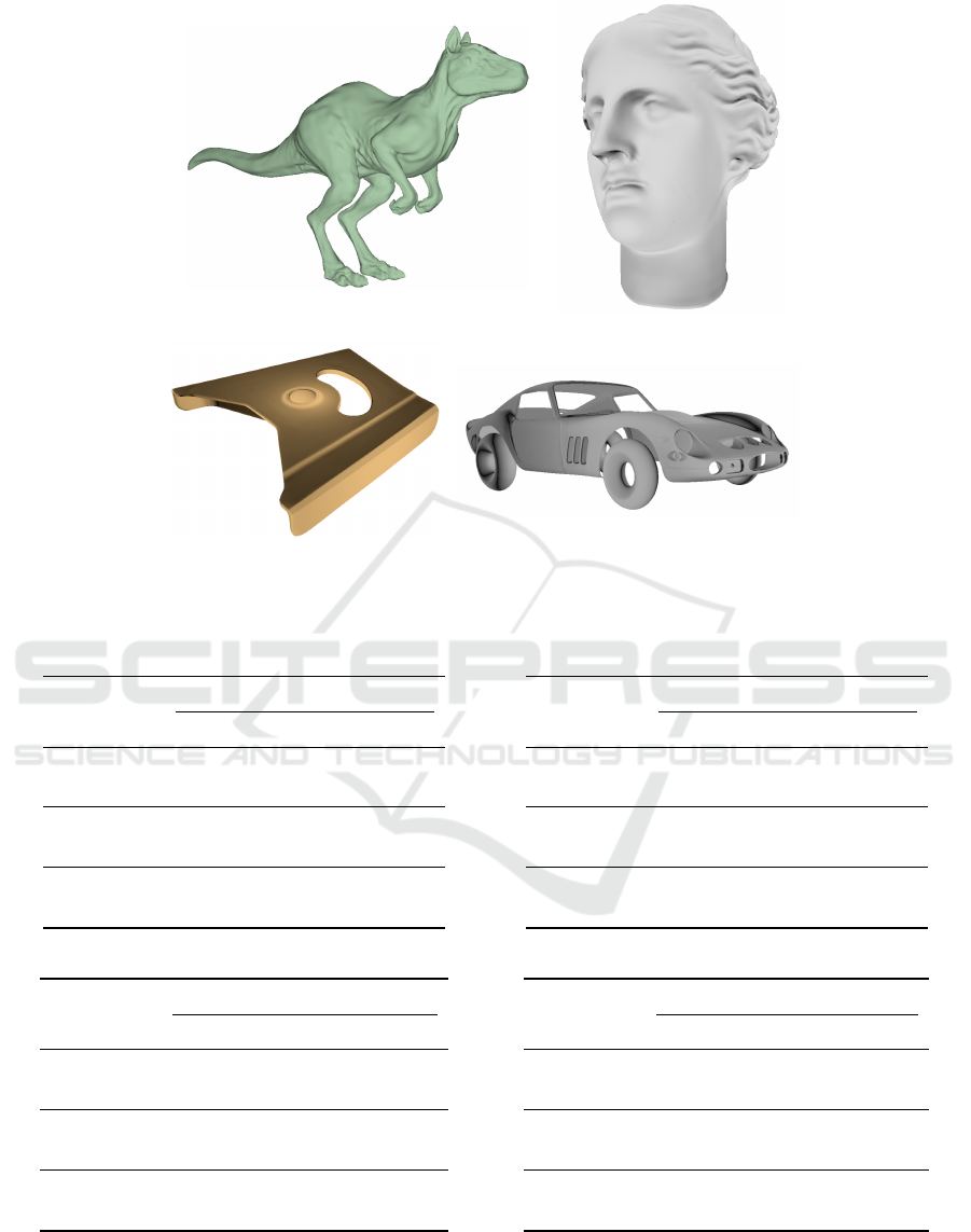
(a) Killeroo

(b) Head

(d) Car

Figure 7: Test models.

Table 2: Thousands of #KS obtained with the different culling techniques for the four test models.

(a) Killeroo

µ = 1 µ = 2 µ = 4

No Culling 1564.79 485.76 178.47

847.16 261.89 95.72

54.14% 53.91% 53.63%

SQC

1564.79 378.63 139.71

100% 77.95% 78.29%

LQC

841.98 259.90 94.82

53.81% 53.5% 53.13%

(b) Head

µ = 1 µ = 2 µ = 4

No Culling 2309.04 742.09 225

1223.83 368.87 131.85

53% 49.71% 58.6%

SQC

1829.71 554.62 199.82

79.24% 47.74% 88.81%

LQC

1211.38 368.28 131.23

52.45% 49.63% 58.33%

µ = 1 µ = 2 µ = 4

No Culling 4245.46 1593.56 576.54

1578.48 716.35 252.02

62.81 % 55.04 % 56.28%

SQC

2977.54 907.97 325.36

29.86% 43.02% 43.56%

LQC

2373.27 716.07 251.76

44.09 % 55.06% 56.33%

(d) Car

µ = 1 µ = 2 µ = 4

No Culling 4448.50 1493.51 607.11

2520.33 839.08 311.96

56.66% 56.18% 51.38%

SQC

3444.57 1149.10 459.18

56.81% 56.22% 55.25%

LQC

2527.32 839.68 335.44

77.43% 76.94% 75.63%

mentation, that has a signiﬁcant degree of divergence,

spoils the advantage achieved by reducing the number

of KSDice to be rendered in cases with similar tessel-

lation factors for all the surfaces, so the frame rate

drops. In this case, the best results are obtained by the

Dice Culling implementation, since the backface KS-

Dice are removed with very simple computations with

no divergence on the GS. Otherwise, the BackPatch

GRAPP 2016 - International Conference on Computer Graphics Theory and Applications

Table 3: PSNR obtained with the different culling techniques for the four test models.

(a) Killeroo

µ = 1 µ = 2 µ = 4

No Culling 44.51 42.95 40.75

DC 44.50 42.95 40.75

SQC 44.53 42.95 40.75

LQC 39.16 38.64 38.22

(b) Head

µ = 1 µ = 2 µ = 4

No Culling 42.37 43.93 42.97

DC 42.36 43.86 42.57

SQC 42.36 43.95 42.57

LQC 38.88 38.41 38.21

µ = 1 µ = 2 µ = 4

No Culling 41.89 41.39 39.77

DC 41.02 41.65 39.94

SQC 41.11 41.42 39.78

LQC 40.60 41.29 39.70

(d) Car

µ = 1 µ = 2 µ = 4

No Culling 38.64 38.35 40.47

DC 38.53 38.34 40.45

SQC 38.54 38.34 40.48

LQC 34.87 34.47 35.25

Table 4: FPS obtained with the different culling techniques for the four test models (speedup against no culling is also shown).

(a) Killeroo

µ = 1 µ = 2 µ = 4

No Culling 27.91 76.14 152.7

DC 26.43 73.1 165.21

0.95x 0.96x 1.08x

SQC 34.46 87.51 162.78

1.23x 1.15x 1.06x

LQC 47.44 107.12 179.9

1.70x 1.41x 1.18x

(b) Head

µ = 1 µ = 2 µ = 4

No Culling 17.90 41.84 113.03

DC 20.66 54.6 158.48

1.15x 1.30x 1.40x

SQC 21.44 49.83 54.56

1.20x 1.19x 0.48x

LQC 33.67 90.24 122.52

1.88x 2.16x 1.08x

µ = 1 µ = 2 µ = 4

No Culling 9.27 27.57 35.22

DC 8.55 26.21 64.94

0.92x 0.95x 1.84x

SQC 15.35 44.49 83.42

1.66x 1.61x 2.37x

LQC 19.01 53.73 100.65

2.05 1.95 2.86

(d) Car

µ = 1 µ = 2 µ = 4

No Culling 10.23 20.31 33.3

DC 9.59 29.91 59.18

0.94x 1.47x 1.77x

SQC 12.85 34.9 58.9

1.26x 1.72x 1.77x

LQC 17.06 44.37 70.56

1.67x 2.18x 2.12x

Culling implementations may still be worthwhile for

values between 300 K and 200 K KSDice in mod-

els such as Killeroo. In this model, there are KSDice

with much higher tessellation factors than others as

they have a greater area in the projected image. These

large KSQuads are an important bottleneck, so perfor-

mance dramatically improves when they are culled.

Thus, 182.7 K KSDice are generated without culling

with µ = 4 for the Killeroo model, achieving 179.9

and 165.21 f ps with the LQC and the DC solutions,

respectively. Therefore, BackPatch Culling attains the

best performance results for the more complex mod-

els, those for which the proﬁt of culling is more no-

ticeable.

Regarding the performance attained with our im-

plementations in the pipeline of current GPUs, Ta-

Efﬁcient Culling Techniques for Interactive Deformable NURBS Surfaces on GPU

100

200

300

400

1 2 4

100

200

300

400

Noculling

LQC

SQC

F P S

(a) Killeroo

100

200

300

400

1 2 4

100

200

300

400

Noculling

LQC

SQC

F P S

(b) Head

100

150

1 2 4

100

150

F P S

Noculling

LQC

SQC

100

1 2 4

100

F P S

Noculling

LQC

SQC

(d) Car

Figure 8: Frame rate with the different culling approaches for the four test models.

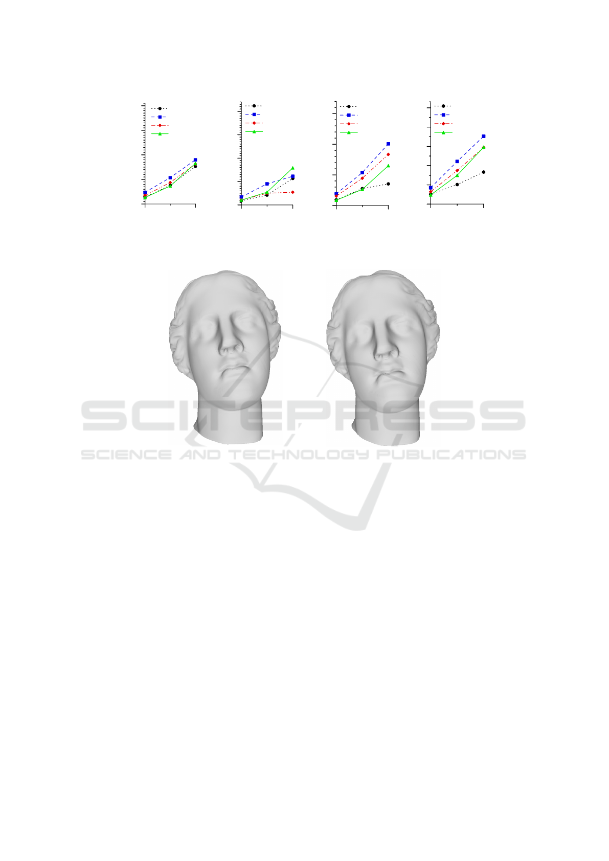
(a)

(b)

Figure 9: Model Head rendered (a) without any culling (b) with culling.

ble 4 shows the good results in terms of frame rate

obtained with µ ≥ 1 for the four test models. These

results are also depicted in the graphs of Figure 8.

The tables and the graphs show that the introduc-

tion of BackPatch culling dramatically improves the

performance of the pipeline, with speed-ups of more

than 2x in the frame rate in some cases, and with-

out decreasing the quality in the rendering, since the

PSNR values are mostly identical. In these cases,

the number of primitives culled in an early stage of

the pipeline is not worth the additional computation

introduced with these backpatch strategies such as

LQC and SQC. Backpatch culling strategies are ap-

plied to KSQuad primitives in an early pipeline stage,

while KSDice primitives are culled out in a latter GPU

pipeline stages in a more classical backface culling

approach. Consequently, backpatch culling strategies

evaluate considerable fewer primitives than the back-

face culling strategy. In any case, the ﬁnal render-

ing obtained by RPNS is a high quality image, as

proved by the PSNR results. Two different renders of

the model Head are shown in Figure 9, without any

culling on the left and with it on the right.

To sum up, the culling techniques proposed in this

work remove an average of around a 20% of the KS-

Dice generated in the case of the SQC method and

over a 41% when the LQC is applied. Both strategies

achieve good results in terms of quality, always over

30 dB, as has previously been mentioned.

6 CONCLUSIONS

In this paper, we provide culling techniques to

NURBS surfaces which cull earlier stage of the

pipeline to reduce as soon as possible the num-

ber of primitives to be processed. Speciﬁcally, we

have developed two new efﬁcient culling techniques,

Lightweight BackPatch Culling (LQC) andStrong

BackPatch Culling (SQC), based on the strong convex

hull property of NURBS surfaces that allows a small

culling overhead compared to the computational sav-

GRAPP 2016 - International Conference on Computer Graphics Theory and Applications

ings, Our proposals have been implemented in Di-

rectX11 to achieve interactive handling of NURBS

surfaces. SQC achieves up to 2.37x speedup over

non-culling proposal whereas LQC up to 2.86x.

As future work, our primary focus is to apply our

culling proposal to handle motion blur rasterization

(Gribel et al., 2013). We also plan to extend our pro-

posal to consider self-collision detection (Wong et al.,

2014).

ACKNOWLEDGEMENTS

This research has been supported by the Gali-

cian Government (Xunta de Galicia) under the

Consolidation Program of Competitive Reference

Groups, cofunded by FEDER funds of the EU (Ref.

GRC2013/055); and by the Ministry of Economy and

Competitiveness of Spain and FEDER funds of the

EU (Project TIN2013-42148-P).

REFERENCES

Akenine-M

oller, T., Haines, E., and Hoffman, N. (2008).

Real-Time Rendering. A. K. Peters.

Claux, F., Barthe, L., Vanderhaeghe, D., Jessel, J.-P., and

Paulin, M. (2014). Crack-free rendering of dynam-

ically tesselated B-rep models. Computer Graphics

Forum, 33(2):263–272.

Cohen, E., Lyche, T., and Riesenfeld, R. (1980). Discrete B-

splines and subdivision techniques in computer-aided

geometric design and computer graphics. Computer

Graphics and Image Processing, 14(2):87–111.

Concheiro, R., Amor, M., and B

oo, M. (2010). Synthe-

sis of B

ezier surfaces on the GPU. In Richard, P.,

Braz, J., and Hilton, A., editors, Proceedings of the

GRAPP’10: International Conference on Computer

Graphics Theory and Applications, pages 110–115.

INSTICC Press.

Concheiro, R., Amor, M., Padr

on, E. J., and Doggett, M. C.

(2014). Interactive rendering of NURBS surfaces.

Computer-Aided Design, 56:34–44.

Gribel, C. J., Munkberg, J., Hasselgren, J., and Akenine-

oller, T. (2013). Theory and analysis of higher-order

motion blur rasterization. In Proceedings of the 5th

High-Performance Graphics Conference, HPG’13,

pages 7–15.

Guthe, M., Bal

azs,

A., and Klein, R. (2005). GPU-based

trimming and tessellation of NURBS and T-Spline

surfaces. ACM Transactions on Graphics, 24(3).

Hasselgren, J., Munkberg, J., and Akenine-M

oller, T.

(2009). Automatic pre-tessellation culling. ACM

Trans. Graph., 28(2):19:1–19:10.

Krishnamurthy, A., Khardekar, R., and McMains, S. (2007).

Direct evaluation of NURBS curves and surfaces on

the GPU. In Proceedings of SPM’07: The 2007 ACM

Symposium on Solid and Physical Modeling, pages

329–334.

Krishnamurthy, A., Khardekar, R., McMains, S., Haller, K.,

and Elber, G. (2009). Performing efﬁcient NURBS

modeling operation on the GPU. IEEE Transactions

on Visualization and Computer Graphics, 15(4):530–

543.

Kumar, S., Manocha, D., and Lastra, A. (1996). Inter-

active display of large-scale NURBS models. IEEE

Transactions on Visualization and Computer Graph-

ics, 2(4):323–336.

Loop, C. T., Nießner, M., and Eisenacher, C. (2011). Effec-

tive back-patch culling for hardware tessellation. In

Proceeding of the VMV 2011: Vision, Modeling, and

Visualization Workshop, pages 263–268.

Munkberg, J., Hasselgren, J., Toth, R., and Akenine-M

oller,

T. (2010). Efﬁcient bounding of displaced B

ezier

patches. In Proceedings of the Conference on High

Performance Graphics, HPG’10, pages 153–162. Eu-

rographics.

Nießner, M. and Loop, C. (2012). Patch-based occlusion

culling for hardware tessellation. In Proceedings of

the Computer Graphics International 2012, CGI’12.

Nießner, M., Loop, C., Meyer, M., and DeRose, T. (2012).

Feature adaptive GPU rendering of Catmull-Clark

subdivision surfaces. ACM Transactions on Graphics,

31(1).

Pﬁster, H., Zwicker, M., van Baar, J., and Gross, M. (2000).

Surfels: surface elements as rendering primitives. In

Proceedings of the SIGGRAPH’00: 27th annual con-

ference on Computer graphics and interactive tech-

niques, pages 335–342, New York, NY, USA. ACM

Press/Addison-Wesley Publishing Co.

Piegl, L. and Tiller, W. (1997). The NURBS Book. Springer.

Sch

afer, H., Nießner, M., Keinert, B., Stamminger, M., and

Loop, C. (2014). State of the art report on real-time

rendering with hardware tessellation. In Eurograph-

ics, State of the Art Reports.

Sederberg, T. W. and Meyers, R. J. (1988). Loop detection

in surface patch intersections. Computer Aided Geo-

metric Design, 5(2):161–171.

Shen, J., Kosinka, J., Sabin, M. A., and Dodgson, N. A.

(2014). Conversion of trimmed NURBS surfaces to

CatmullClark subdivision surfaces. Computer Aided

Geometric Design, 13(7–8):486–498.

Shirman, L. A. and Abi-Ezzi, S. S. (1993). The cone of nor-

mals technique for fast processing of curved patches.

Computer Graphics Forum, 12(3):261–272.

Smith, J. and Schaefer, S. (2015). Selective degree elevation

for multi-sided B

ezier patches. Computer Graphics

Forum, 34(2).

Wong, S.-K., Lin, W.-C., Wang, Y.-S., Hung, C.-H., and

Huang, Y.-J. (2014). Dynamic radial view based

culling for continuous self-collision detection. In Pro-

ceedings of the 18th meeting of the ACM SIGGRAPH

Symposium on Interactive 3D Graphics and Games,

I3D’14, pages 39–46.

Yeo, Y. I., Bin, L., and Peters, J. (2012). Efﬁcient pixel-

accurate rendering of curved surfaces. In Proceedings

of the i3D’12: ACM SIGGRAPH Symposium on Inter-

active 3D Graphics and Games, pages 165–174, New

York, NY, USA. ACM.

Efﬁcient Culling Techniques for Interactive Deformable NURBS Surfaces on GPU