
Multi-Class Error-Diffusion with Blue-noise Property
Xiaoliang Xiong, Haoli Fan, Jie Feng, Zhihong Liu and Bingfeng Zhou
Institute of Computer Science and Technology, Peking University, 100871, Beijing, China
Keywords:
Sampling, Error-Diffusion, Halftoning, Image Vectorization, Blue-noise.
Abstract:
Existing researches on error-diffusion mainly focus on sampling over a single channel of input signal. But
there are cases where multiple channels of signal need to be sampled simultaneously while keeping their
blue-noise property for each individual channel as well as their superimposition. To solve this problem,
we propose a novel discrete sampling algorithm called Multi-Class Error-Diffusion (MCED). The algorithm
couples multiple processes of error-diffusion to maintain a sampling output with blue-noise distribution. The
correlation among the classes are considered and a threshold displacement is introduced into each process of
error-diffusion for solving the sampling conflicts. To minimize the destruction to the blue-noise property, an
optimization method is used to find a set of optimal key threshold displacements. Experiments demonstrate
that our MCED algorithm is able to generate satisfactory multi-class sampling output. Several application
cases including color image halftoning and vectorization are also explored.
1 INTRODUCTION
Error-diffusion (ED) is originally a halftoning tech-
nique that quantizes a multi-level image to a binary
one while preserving its visual appearance through
diffusing the quantization error of one pixel to its
neighborhood (Floyd and Steinberg, 1976). It is
widely used in the industry of printing and displaying,
and also an important sampling algorithm working on
discrete domain. Some researchers extend its usage
into digital geometry processing (Alliez et al., 2002).
Previous research mainly focused on the behavior
of error-diffusion sampling over a single channel of
input signal (Ulichney, 1988; Ostromoukhov, 2001;
Zhou and Fang, 2003; Chang et al., 2009). However,
there are cases where multiple channels of input sig-
nal need to be sampled simultaneously, while certain
ideal properties such as blue-noise are also required
for all the sampling output of these channels.
Simply overlapping the output of blue-noise sam-
pling for multiple individual channels can not guaran-
tee the blue-noise property of their superimposition.
Hence, we are aiming to propose a novel Multi-Class
Error-diffusion (MCED) algorithm to solve this prob-
lem. Here, a class refers to the sampling process for a
single channel of input signal as well as its sampling
output. For an ideal multi-class error-diffusion with
This work is partially supported by NSFC grants
#61170206, #61370112.
blue-noise property, the following requirements must
be satisfied:
1. The sampling point distribution of each individual
class should possess blue-noise property.
2. When the sampling output of all the classes are
superimposed, no two sampling points from dif-
ferent classes can occupy the same position.
3. When all the sampling points from all the classes
are superimposed and considered as a whole, their
distribution should possess blue-noise property.
The first requirement is naturally guaranteed by
the standard ED algorithm. For the second, we
remain only one class with the highest priority and
disable the others when conflict occurs. However,
the selection of a certain class may disrupt the point
distribution of other classes which violates the first
requirement. To solve this problem, we introduce a
threshold displacement into each process of ED and
they are optimized to minimize the destruction to the
blue-noise property. Since the frequency spectrum
property of each class and the final output is consid-
ered during the threshold displacement optimization,
the blue-noise property is promised after all classes
are superimposed (the third requirement). After meet-
ing these requirements, our MCED algorithm gener-
ates satisfactory multi-class sampling output.
Contribution. The contributions of of our work
includes: (1) Proposing a multi-class error-diffusion
28
Xiong, X., Fan, H., Feng, J., Liu, Z. and Zhou, B.
Multi-Class Error-Diffusion with Blue-noise Property.
DOI: 10.5220/0005677300260036
In Proceedings of the 11th Joint Conference on Computer Vision, Imaging and Computer Graphics Theory and Applications (VISIGRAPP 2016) - Volume 1: GRAPP, pages 28-38
ISBN: 978-989-758-175-5
Copyright
c
2016 by SCITEPRESS – Science and Technology Publications, Lda. All rights reserved

framework, the validity of which can be explained
by the commonly used Fourier transform (Knox and
Eschbach, 1993); (2) Giving a parameter optimiza-
tion method to ensure the blue-noise property of
the output. Experiment results using these optimal
parameters show the effectiveness of the method;
(3) Several applications of the MCED are explored,
showing that our algorithm is generic and applicable
in many areas in computer graphics.
2 RELATED WORK
The original ED is an algorithm invented for gray-
scale image displaying and printing (Floyd and Stein-
berg, 1976). It is also frequently used in many other
areas in computer graphics as a sampling algorithm
(Alliez et al., 2002; Bourguignon et al., 2004; Kim
et al., 2009). Its principle is shown inside the dashed
line of Fig.1. In this algorithm, each pixel p(x,y) ∈
[0,1] in the input image p is parsed with a serpentine
scan line order and quantized by a quantizer:
Q(p
,
,u) =
(
1, p
,
> u
0, otherwise
(1)
After that, the quantization error e(x, y) is calculated
and distributed into multiple unparsed pixels by accu-
mulating to an error buffer b(·,·), which is used to
compensate the error. Therefore, for pixel p(x,y),
the actual input p
,
to the quantizer Q(·,·) is p
,
=
p(x,y) + b(x, y). Here, the error filter a
jk
is a set of
constant coefficients, and the quantization threshold u
in Q(·,·) is also a fixed value, e.g. u = 0.5.
Some important improvements to the original ED
algorithm include the introduction of a variable error
filter (Ostromoukhov, 2001) and a variable threshold
value (Zhou and Fang, 2003) to ensure the blue-
noise property of the sampling output. In this paper,
we use Zhou and Fang’s threshold modulated ED
algorithm to build our MCED framework. Similar as
in (Chang et al., 2009), we refer to that algorithm as
the standard ED, and its diagram is given by Fig.1 as
a whole. Unlike the original ED, the threshold u and
the error filter a
jk
here are not constant, but functions
of the input pixel p = p(x,y), that is, u = 0.5 + r(p),
and a
jk
= a
jk
(p). Here, r(p) = δ(p) · λ(x, y) is a
modulated white noise. The modulation strength δ(p)
for the white noise λ(x,y), and the error filter a
jk
(p)
are pre-optimized so that the output of the standard
ED possesses blue-noise property.
Some mathematical analysis about the behavior of
error-diffusion is given in (Weissbach and Wyrowski,
1992; Knox and Eschbach, 1993), which helps to
explain and predict the result of many techniques
Q(p’, u)p(x, y) c(x, y)
Error filter:a
jk
+
+
+
−
p’
u
+
0.5
r(p)
Details of standard E-D 4-1
b(x,y)
a
jk
(p)
e(x,y)
Original error diffusion
Error
buffer
b(j,k)
Figure 1: The principle of the standard error-diffusion.
derived from the original ED algorithm. Ulichney
first proposed the concept of blue-noise (Ulichney,
1988) and used it as a tool to measure the quality of
ED output. For single-class ED, some ideal results
have been achieved for generating sampling points
with such a property (Ostromoukhov, 2001; Li and
Allebach, 2001; Zhou and Fang, 2003).
Using ED to sample multiple channels of input
signals in a coordinated way is not a novel problem. It
traditionally exists in the area of color printing, where
a limited number of colorants are used to reproduce
a continuous-tone color image (Baqai et al., 2005).
Many studies focus on solving this problem using
ED technique, which is called vector error-diffusion
in some literature, because they quantized the input
signals simultaneously by treating them as a vector
(Haneishi et al., 1996; Kang, 1999; Damera-Venkata
et al., 2003). For example, the vector ED algorithm
proposed in (Damera-Venkata and Evans, 2001) uses
an optimum matrix-valued error filter to take into
account the correlation among color planes. It can
generate sampling output with blue-noise property for
color images, but cannot guarantee this property for
each individual color channel.
Wei extends the traditional Poisson disk sampling
for a single channel of signal into a multi-class blue-
noise sampling algorithm (Wei, 2010). The algorithm
is able to sample a set of input signals in a correlated
way while keeping the blue-noise property of the
whole output. It can also precisely control the number
or density of the generated sampling points. Unlike
the ED which works directly in a discrete domain,
this algorithm is originally designed in a continuous
domain. Hence it is not suitable to be applied
in certain application areas that deal with discrete
domain, such as color image halftoning (Wei, 2012).
3 MULTI-CLASS
ERROR-DIFFUSION
Our MCED algorithm mainly concerns about simul-
taneously sampling on multiple channels of input
signals and maintaining the blue-noise property for all
the classes as well as their superimposition. If simply
performing the standard ED independently on each
Multi-Class Error-Diffusion with Blue-noise Property
29
...
...
E
n
p
n
E
2
p
2
E
1
p
1
E
0
p
0
Q
n
p
n
Q
2
p
2
Q
1
p
1
Q
0
p
0
...
d
0
d
1
Disable
control
c
0
c
1
c
2
c
n
𝑐
0
0
𝑐
1
0
𝑐
2
0
𝑐
𝑛
0
Disable
control
d
11
d
12
d
1n
+
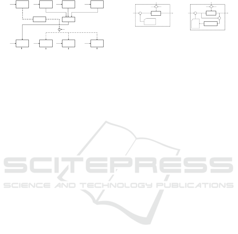
s
i
Figure 2: The framework of our MCED algorithm, where
{p
i
|i = 1, ··· , n} are the input signals, and p
0
=
∑
n
i=1
p
i
is
an internal reference signal. After two processing steps of
modified standard ED, Q
i
and E
i
, the framework generates
blue-noise sampling outputs {c
i
|i = 0, · ·· ,n}. The pseudo
code for the framework can be found in the appendix.
channel of input signal, there may be sampling points
from different classes situated at the same sampling
position when they are superimposed, which is called
sampling conflict. Hence, the blue-noise property of
the superimposed output cannot be guaranteed. To
solve this problem, we first perform the quantization
on each channel of signal, and produce a set of initial
sampling outputs with sampling conflicts. Then, the
conflicts are removed by disabling the outputs of
certain classes based on the inter-class correlation. In
this way, the initial outputs are modified to generate
the final sampling points. During the process of quan-
tization and error-diffusion, a threshold displacement
is introduced to decrease the occurrence of sampling
conflict and maintain the blue-noise property.
3.1 MCED Framework
Fig.2 illustrates the framework of our MCED algo-
rithm. It takes n channels of signals {p
i
|i = 1,·· · ,n}
as input, where p
i
= p
i
(x,y) is a 2-D discrete function
that satisfies p
i
(x,y) ∈ [0,1] and
∑
n
i=1
p
i
(x,y) ≤ 1.
In fact, it defines the density of sampling points to
be generated at the spatial position (x,y). Specially,
when p
i
represents an image, element p
i
(x,y) is the
intensity of the pixel at position (x, y). Our framework
concerns the processing of individual channels of
signals as well as their correlations, and produces
corresponding sampling point sets {c
i
|i = 1, · ·· ,n},
where c
i
(x,y) = 1 indicates a sampling point gener-
ated at (x, y) for signal p
i
, while 0 means no point
generated. Therefore, the sampling process from the
input p
i
to the output c
i
is referred as a class C
i
.
To facilitate the inter-class correlation, we define
a special internal signal p
0
, whose sampling density
is p
0
(x,y) =
∑
n
i=1
p
i
(x,y). Sampling to p
0
with the
standard ED, we can also obtain a blue-noise output,
which is used as a reference for the superimposition
of the sampling output of all the classes. That means
Q
i
(p’, u)p
i
(x, y) c
i
(x, y)
+
p’
u
+
0.5
r(p)
b
i
(x,y)
Error buffer
b
i
(∙, ∙)
m
i
Q
i
(p’, u)p
i
(x, y) c
i
(x, y)
Error filter
+
+
+
−
p’
u
+
0.5
r(p)
b
i
(x,y)
Error
buffer
b
i
(∙, ∙)
m
i
Figure 3: Two processing steps of modified ED: Q
i
(left)
performs only the quantization and E
i
(right) complete the
final error-diffusion (i = 0,...,n).
the corresponding output of p
0
, denoted as c
0
, will be
identical to the superimposition of {c
i
|i = 1, ··· ,n}.
Hence, we name C
0
as a reference class.
Our framework parses the elements {p
i
(x,y)|i =
0,··· ,n} in a serpentine scan line order. All p
i
(x,y) at
the same position (x,y) are processed simultaneously,
and then the processing moves to the next position.
For each group of {p
i
(x,y)|i = 0,··· ,n} at (x,y), the
processing of each class includes two steps: Q
i
and
E
i
. Q
i
performs independent sampling and produces
initial output c
0
i
(x,y) for each individual class C
i
;
while E
i
modifies the initial output according to the
correlation between the sampling classes and generate
the final output c
i
(x,y).
3.2 Quantization and Error-Diffusion
The work flow of the two processing steps, Q
i
and E
i
,
are shown in Fig.3. Acturally, E
i
is a modified version
of the standard ED given in Fig.1. It simply adds one
more variable m
i
to the latter’s quantization threshold.
This simple modification plays an important role in
our framework, because m
i
will be used to introduce
the inter-class correlation into the sampling, and that
is the key to avoid sampling conflict and ensure the
blue-noise property of c
i
.
It is notable that Q
i
produces only the initial sam-
pling output, hence it performs only the quantization
part of E
i
. Although Q
i
shares the error buffer b
i
(·,·)
with E
i
, it does not modify b
i
(·,·). This is because
the output of Q
i
will be modified in E
i
and thus the
quantization error made in the latter step is the one
that is to be distributed for the further processing.
3.3 Removing Sampling Conflicts
In our framework, the input signal p
i
, i = 0,··· ,n, of
each class is firstly processed by Q
i
, and generates
corresponding uncorrelated blue-noise output c
0
i
. In
order to eliminate the conflict after superimposition,
the correlation between classes are introduced by the
reference class C
0
. Based on that, some classes with
sampling conflicts will be disabled, i.e. they will be
prohibited to produce a sampling point.
As shown in Fig.4, when Q
0
of class C
0
does not
generate a sampling point at current position (x,y),
GRAPP 2016 - International Conference on Computer Graphics Theory and Applications
30

{Q
i
} have
output?
{Q
i
} have
conflicts?
Disable all E
i
Disable E
0
No adjustment
needed
(ideal output)
Outputs of Q
i
Q
0
has output?
N Y
N
N
Y
Y
E
i
d
0
d
1
d
1
+s
i
Disable some of E
i
,
only one remains
Figure 4: Eliminating sampling conflicts by disabling some
of the classes.
the output of all {E
i
|i 6= 0} should be forced to be 0. In
other words, all E
i
should be disabled from generating
a sampling point at (x, y), for there is no correspon-
dence in the final superimposition. Similarly, when
Q
0
generates sampling point but none of {Q
i
|i 6= 0}
does, E
0
should also be disabled because no E
i
will
provide sampling point to form this superimposition.
The third case, in which {Q
i
|i 6= 0} generate sampling
points without conflicts, is the ideal case that we are
expecting and no modification to {c
0
i
|i 6= 0} is needed.
Finally, when sampling conflicts occur (
∑
j6=0
c
0
j
> 1),
most of the conflicting classes must be disabled, and
only one of them with the highest priority is allowed
to remain. Here, we give the priority to the class C
k
with the highest average sampling density, i.e. k =
argmax
j
∑
(x,y)
p
j
(x,y), for j 6= 0 and c
0
j
= 1. Then,
a binary selecting signal s
i
(i 6= 0) is defined, where
s
i
= 0 means E
i
should be disabled:
s
i
=
0,
∑
j6=0
c
0
j
> 1 and i 6= k;
1,
∑
j6=0
c
0
j
> 1 and i = k;
1,
∑
j6=0
c
0
j
≤ 1.
(2)
To disable a class, we utilize another disabling
signal to modify the quantization threshold. It is
based on an important fact about the ED: If the thresh-
old u in the quantizer Q(p
,
,u) takes a value larger than
any possible value of input p, the output of Q will be
forced to be 0, and the corresponding class will be
disabled. As shown in Fig.2, the disabling signals are
obtained based on the initial outputs {c
0
i
|i = 0,· · · ,n}
by the Disable control, where d
0
= ¬(c
0
1
∨ c
0
2
··· ∨ c
0
n
)
and d
1
= ¬(c
0
0
). Then, combining with the selecting
signal s
i
, d
1
turns into a d
1i
= d
1
∧ s
i
for each E
i
(i 6=
0). Therefore, if d
0
/d
1i
= 1, a large value (+∞) will
be added to the corresponding quantization threshold,
and the class will be disabled.
In this way, d
0
, d
1
and s
i
facilitate the correlation
described in Fig.4. For example, when c
0
0
= 1 and
c
0
i
= 1 (i 6= 0), we have d
0
= 0 and d
1
= 0, and
the output of E
i
will be decided by its priority: if
s
i
= 0, E
i
will be disabled. After the class disabling,
sampling conflicts can be removed and no more than
one sampling point will be generated at each position.
3.4 Maintaining Blue-noise Property
Modifying the output of certain Q
i
to remove the
sampling conflicts may cause the destruction of the
blue-noise property of the initial outputs. To solve
this problem, we make use of another important
fact for ED: For a given input signal, a constant
variation of the quantization threshold u will change
the distribution of output sampling points, but will not
affect the average sampling density, as long as u is
not constantly +∞. This fact can be proofed with
the analysis tool provided in (Knox and Eschbach,
1993), which will be briefly described in section
7. Therefore, adding a properly chosen threshold
displacement t
i
to the threshold u will help to decrease
the chance of the sampling conflict occurrence and
restore the blue-noise distribution. The detail of t
i
will
be discussed in the next section.
Hence, the disabling signals d
0
/d
1i
, along with
the threshold displacement t
i
, are finally added to the
thresholds of E
i
via the modification term m
i
in the
second step. Then, E
i
quantizes the input element
p
i
(x,y) at current position (x, y), and the quantization
error is distributed and accumulated to the error buffer
b( j, k). The above processing is repeated during the
parsing of the input elements. When all the elements
p
i
(x,y) are parsed, the final blue-noise MCED output
c
i
that satisfies all the requirements given in Section 1
can be generated.
4 THRESHOLD DISPLACEMENT
After the first step of the MCED, the output of some of
the classes is disabled due to sampling conflicts. This
may disrupt the blue-noise property that originally
existed in the standard ED output. We solve this
problem by adding a constant displacement value t
i
to the quantization threshold for the input p
i
, since a
shift of the threshold may change the distribution of
sampling points and thus may decrease the chance of
sampling conflicts. Therefore, it is possible to ensure
a better blue-noise output with a properly chosen t
i
.
4.1 Displacement Optimization
Our goal is to find a set of optimal threshold displace-
ments {t
i
|i = 0,1,··· ,n}, to decrease the probability
Multi-Class Error-Diffusion with Blue-noise Property
31
of sampling conflict occurrence. Since the sampling
conflict is a interference among all the classes, the
value of the displacement t
i
is related to all the
input signals {p
i
|i = 1,··· ,n}. For each class C
i
,i =
0,··· ,n, in a n-class MCED, we treat the influence
from all other sampling classes as a noise, which is
characterized by its strength σ
i
=
∑
j6=0∧ j6=i
p
j
. We
assume that the same amount of σ
i
for a given p
i
will result in similar output. Since σ
i
can be derived
from σ
i
= p
0
− p
i
, then t
i
can be simplified as a
function of p
i
and p
0
. As class C
0
is designed as a
reference for the superimposition of other n classes, t
0
is related with only the sum of other classes inputs, i.e.
p
0
=
∑
n
i=1
p
i
. Therefore, given an input combination
(p
0
, p
i
),i = 1, ··· ,n, in a n-class MCED, we have:
(
t
i
= g(p
0
, p
i
),i = 1,··· , n,
t
0
= f (p
0
).
(3)
Then, optimal t
i
are calculated by solving an op-
timization problem. The optimization target function
is defined according to the Fourier power spectrum of
the sampling output. Based on the existing research
(Ulichney, 1988; Zhou and Fang, 2003), the blue-
noise property of a sampling set can be measured by
the anisotropy and the lower frequency ratio of its
spectrum. In this paper, the sampling output of ED are
affected by both the input signal p
i
and the threshold
displacement t
i
. Therefore, the anisotropy α(p
i
,t
i
)
and lower frequency ratio β(p
i
,t
i
) for the final output
c
i
can be modified from their original formulations in
(Zhou and Fang, 2003):
(
α(p
i
,t
i
) = Corre(P
0
(p
i
,t
i
),P
45
(p
i
,t
i
),P
90
(p
i
,t
i
)),
β(p
i
,t
i
) = L(p
i
,t
i
),
(4)
where Corre(·) is a cross-correlation function; P
0
(·),
P
45
(·) and P
90
(·) are segmented radially averaged
power spectrums; L(·) is the lower frequency ratio.
Therefore, our target function T to be minimized
in the searching of optimal threshold displacements t
i
is defined as:
T = ω
1
·
ω
0
·
N
∑
i=1
α(p
i
,t
i
) + (1 − ω
0
) ·
N
∑
i=1
β(p
i
,t
i
)
!
+(1 − ω
1
) · (ω
0
· α(p
0
,t
0
) + (1 − ω
0
) · β(p
0
,t
0
)),
(5)
where the weights ω
0
= 0.5 and ω
1
= 0.7 are taken
in our implementation. A simplex method (Press
et al., 1992) is adopted to automatically search for the
optimal displacement {t
i
|i = 0,1,·· · ,n}.
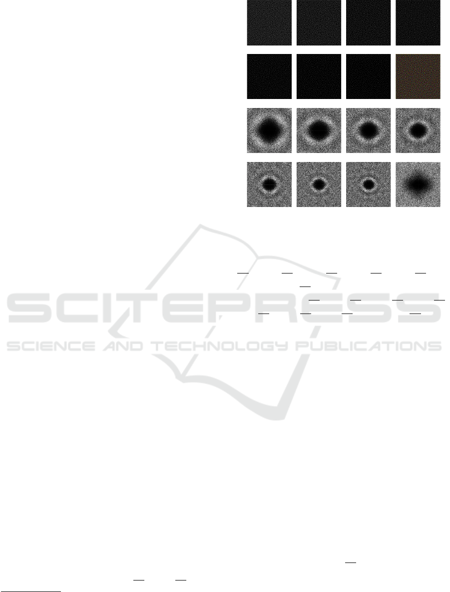
Fig.5
1
demonstrates an example of the displace-
ment optimization. Given p
1
=
32
255
, p
2
=
21
255
, p
3
=
1
Config the PDF reader with 100% scaling ratio and the
given DPI for best viewing of the details, similar for the
following figures.
(a) C
1
(b) C
2
(c) C
3
(d) C
4
(e) C
5
(f) C
6
(g) C
7
(h) C
0
(i) C
1
(j) C
2
(k) C
3
(l) C
4
(m) C
5
(n) C
6
(o) C
7
(p) C
0
Figure 5: Optimization result for a 7-class ED. (a)-(h)
Sampling outputs of each classes C
i
. (i)-(p) Corresponding
Fourier power spectra. (Image best viewed at 306 DPI).
16
255
, p
4
=
12
255
, p
5
=
8
255
, p
6
=
6
255
, p
7
=
5
255
, and
p
0
=
∑
i6=0
p
i
=
100
255
, the optimized threshold displace-
ments are: t
1
=
34
255
, t
2
=
18
255
, t
3
=
52
255
, t
4
=
23
255
,
t
5
=
80
255
, t
6
=
46
255
, t
7
=
17
255
, and t
0
= −
9
255
. The
sampling outputs of classes {C
i
|i = 0, · ·· ,7}, and
their corresponding Fourier power spectra are given in
the figure. Fig.5(h) is the superimposition of the dots
from the 7 classes, which are colored in red, green,
blue, yellow, magenta, cyan and white, respectively.
The optimization is performed on 256 × 256 patches.
4.2 Displacement Interpolation
To decrease computational costs, we perform dis-
placement optimization only on a set of selected key
input combinations, by minimizing the target function
T in Eq.5. Then, the optimal threshold displacements
for other input combinations can be calculated by
interpolation, where t
i
= g(p
0
, p
i
), i = 1,··· , n, is
implemented with a bilinear interpolation, and t
0
=
f (p
0
) with a 1-D linear interpolation.
The key input combinations and their correspond-
ing optimal threshold displacement values are shown
in the tables contained in Fig.6. The key levels are
selected by an interval of
16
255
. For convenience, all
the numbers filled into the table are 255 times of their
real values. The right table gives the correspondence
between the threshold displacement t
0
and the input
p
0
of the reference class C
0
, as t
0
= f (p
0
). The left
table is composed of two parts:
GRAPP 2016 - International Conference on Computer Graphics Theory and Applications
32

0 16 32 48 64 80 96 112 128 144 160 176 192 208 224 240 255
p
0
p
i
0 0 0
16 0 0 16
32 0 39 0 32
48 0 49 -3 0 48
64 0 14 51 -23 0 64
80 0 28 35 3 37 0 80
96 0 56 18 43 6 -6 0 96
112 0 49 30 53 96 12 59 0 112
128 0 34 10 11 62 -26 2 93 0 128
144 0 6 26 59 5 -1 12 18 14 0 144
160 0 14 100 106 12 56 44 98 90 22 0 160
176 0 12 43 47 42 48 39 100 52 25 47 0 176
192 0 -46 28 6 0 -7 45 -36 0 25 37 1 0 192
208 0 75 54 -7 71 -33 59 23 -1 13 9 13 0 0 208
224 0 12 18 89 12 -2 75 0 0 0 12 3 0 50 0 224
240 0 16 12 9 9 12 49 -20 -2 14 50 1 9 50 46 0 240
255 0 12 12 20 12 0 29 12 44 50 18 0 50 43 50 86 0 255
p
0
p
i
0 16 32 48 64 80 96 112 128 144 160 176 192 208 224 240 255
1
p
0
t
0
0 0
16 0
32 65
48 -35
64 -39
80 -90
96 -20
112 -15
128 -79
144 0
160 169
176 13
192 61
208 109
224 168
240 166
255 64
1
Figure 6: Threshold displacement t
0
and t
i
with their Fourier analysis results for different key input combinations (p
0
, p
i
).
For convenience, the numbers in this table are all 255 times of the value by their definition.
(a)
(b)
(c)
(d)
(e)
(f)
Figure 7: Two-class ED with density changing horizontally
in opposite directions: in (a)-(c) from
255
255
to 0, and in (d)-
(f) from
51
255
to 0. (a)&(d) are the superimposition, (b)&(c)
and (e)&(f) are the sampling points for the two classes,
respectively. (Image best viewed at 150 DPI).
• The values of the threshold displacement t
i
=
g(p
0
, p
i
) for the given key input combinations are
enumerated in the lower-left triangle area. They
are obtained by solving the optimization problem
of Eq.5. The indices of p
0
and p
i
are given in the
bottom row and the leftmost column, respectively.
• The corresponding power spectra of the sampling
outputs for p
i
and p
0
can be found in the upper-
right triangle area, where the left image is for p
i
and the right for p
0
. The indices of p
0
and p
i
are given in the top row and the rightmost col-
umn. The power spectra show that, for the given
input combinations, our optimization successfully
converges to threshold displacements that can
produce outputs with ideal blue-noise property.
Hence, the threshold displacement of a key input
combination can be read directly from the table.
For example: given p
0
=
112
255
and p
i
=
16
255
, the
displacement value t
i
= g(
112
255
,
16
255
) =
49
255
can be
found in the cell at the 8th row and the 2nd column
of the left table, and the corresponding power spectra
are in the cell at the 2nd row and 8th column.
Then, for arbitrary combination (p
0
, p
i
) that is
not included in Fig.6, we use a bilinear interpolation
to obtain their t
0
and t
i
. For example, for an input
(p
0
, p
i
) = (
122
255
,
21
255
), its t
i
is interpolated between four
key values g(
112
255
,
16
255
), g(
112
255
,
32
255
), g(
128
255
,
16
255
) and
g(
128
255
,
32
255
) that exist in the table. The value of t
0
is
interpolated in a similar way, but using a 1-d linear
interpolation between the values in the right table.
Fig.7 gives two groups of experiment results of a two-
class MCED using our key values and interpolation
mechanism. It can be seen that the sampling results
meet the requirement of MCED given in Section 1.
5 EXPERIMENTAL RESULTS
We proposed a multi-class ED algorithm that is able
to produce blue-noise sampling points on multiple
input signals as well as their superimposition. Given
k channel of signals, each with n elements, the time
complexity of our algorithm (Alg.1) is O(kn). Some
experimental results have been shown in Section 4.
In this section, we compare our MCED with the
per-channel standard ED (Zhou and Fang, 2003), and
our method achieves results significantly better than
the latter. As illustrated in Fig.8(b)-(g), applying
our MCED to three channels of input signal, three
sampling point sets with blue-noise distribution can
be produced (Fig.8(b)(d)(f), colored with red, green
and blue for distinction). The corresponding Fourier
power spectra in Fig.8(c)(e)(g) demonstrate the per-
fect blue-noise property of each class. Fig.8(a) is a
colored superimposition of the three classes. Since
Multi-Class Error-Diffusion with Blue-noise Property
33
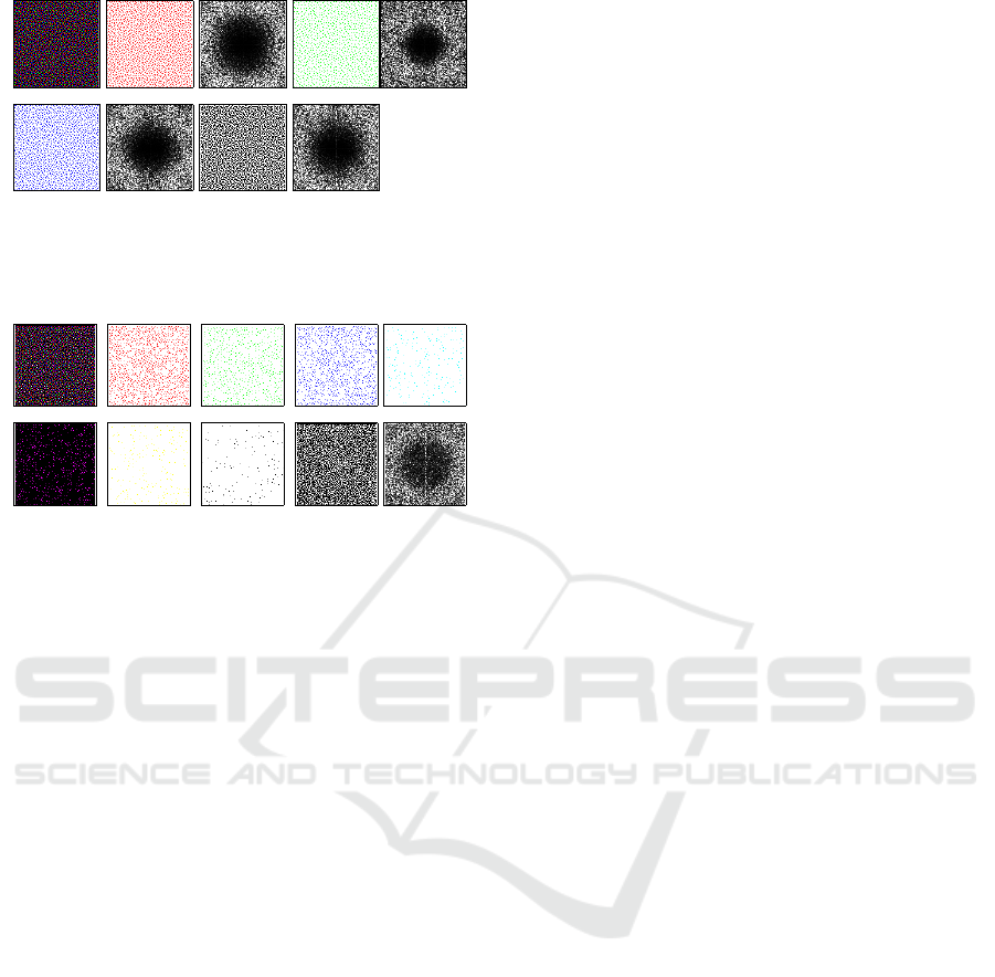
(a) (b) (c) (d) (e)
(f) (g) (h) (i)
Figure 8: A 3-class MCED sampling result. Each individual
class (b-g) and their superimposition (h-i) possess perfect
blue-noise property. (Best viewed at 150 DPI).
(a) (b) (c) (d) (e)
(f) (g) (h) (i) (j)
Figure 9: A 3-class sampling using standard ED. Large
number of conflicting sampling points exists (e-h), and the
superimposition does not possess blue-noise property (i-j).
(Best viewed at 150 DPI).
no sampling conflicts exist, i.e., none of the sampling
point overlaps with others, there are no color other
then red, green and blue in the image. Fig.8(h)-(i)
show that the superimposed point sets also possesses
blue-noise property.
On the contrary, if applying the standard ED to
each channel of signal separately, though each set of
sampling points has blue-noise distribution, a large
number of sampling conflicts will occur when the
three point sets are superimposed. Fig.9(a) is also a
colored superimposition of the sampling point sets,
where each color channel correspond to a class. Then,
in Fig.9(b)-(d) are the sampling points that do not
overlap with others, and Fig.9(e)-(h) show the con-
flicting sampling points, generated by the overlapping
of points from different classes (The colors indicate
the combination). Consequently, the superimposition
set can not maintain blue-noise property (Fig.9(i)-(j)).
The sampling conflicts are harmful in certain
application areas, such as color printing. For the per-
channel ED, uncontrollable overlapping of sampling
points will affect the controlling of the maximum ink
amount at each position, and the final printing quality.
Our MCED method can help to solve this problem
and hence brings an important improvement.
6 APPLICATIONS
6.1 MCED for Color Image Halftoning
ED algorithm is widely used in grayscale image
halftoning due to its ideal blue-noise property (Os-
tromoukhov, 2001; Zhou and Fang, 2003). For color
image halftoning, a commonly used way is to perform
standard ED independently on each color plane, and
then superimpose the results to create a color halfton-
ing. Since halftoning dots for each color plane are
generated independently, the blue-noise property for
their superimposition can not be guaranteed. This
may result in uncontrolled color appearance in the
generated halftone image (Fig.10(p)).
In this section, we utilize our MCED to generate
color halftone images that meet the requirements: The
distribution of the halftone dots with the same color
should possess blue-noise property; The distribution
of all the dots contained in the halftone image as a
whole should also possess blue-noise property.
6.1.1 15-Class ED for CMYK Color Halftoning
CMYK Color Images. In the state-of-the-art color
printing systems, the device-independent colors are
converted to the densities of the ink dots in four
primary colors: Cyan, Magenta, Yellow and Black.
We denote them as well as their densities as D
1
, D
2
,
D
3
, D
4
, respectively, and they are the input of the
halftoning algorithms. When the output halftoning
image is printed using the four color inks, the dots
generated on paper will appear in totally 15 colors,
corresponding to all possible ink overprints.
If
∑
4
i=1
D
i
> 1 within a local area in a CMYK
halftone image, there must be dots with different
primary colors placed at the same position, and new
colors will be created. The colors generated by 2
primary colors, namely the 2nd order colors, are
denoted as C
12
, C
13
, C
14
, C
23
, C
24
, C
34
. The subscript
indicate the overprinted primary colors, e.g., C
12
is
an overprinting of D
1
and D
2
. In the six colors,
C
12
, C
13
and C
23
correspond to blue, green and red
respectively, and the remaining are very dark colors
because they contain black. Similarly, the 3rd and the
4th order colors generated by 3 or 4 primary colors
are denoted as C
123
, C
124
, C
134
, C
234
, C
1234
. Specially,
the subsets of halftone dots generated by only one
primary color are denote as C
1
, C
2
, C
3
, C
4
.
Without ambiguity, we use the same notations for
the dot density and the sampling class for each color.
Hence, there is a total of 15 classes to be sampled
in MCED. Before applying our MCED in CMYK
color halftoning, the densities of the 15 classes need
GRAPP 2016 - International Conference on Computer Graphics Theory and Applications
34
to decided.
Linear Programming for Dot Densities. For a color
image pixel with
∑
4
i=1
D
i
≤ 1, the dot densities are
simply C
1
= D
1
, C
2
= D
2
, C
3
= D
3
, C
4
= D
4
, and the
densities for higher order colors are 0. While for a
pixel with
∑
4
i=1
D
i
> 1, the dot densities must satisfy:
C
1
+ C
2
+ C
3
+ C
4
+C
12
+ C
13
+ C
14
+ C
23
+ C
24
+ C
34
+C
123
+ C
124
+ C
134
+ C
234
+ C
1234
= 1,
C
1
+ C
12
+ C
13
+ C
14
+ C
123
+ C
124
+ C
134
+ C
1234
= D
1
,
C
2
+ C
12
+ C
23
+ C
24
+ C
123
+ C
124
+ C
234
+ C
1234
= D
2
,
C
3
+ C
13
+ C
23
+ C
34
+ C
123
+ C
134
+ C
234
+ C
1234
= D
3
,
C
4
+ C
14
+ C
24
+ C
34
+ C
124
+ C
134
+ C
234
+ C
1234
= D
4
.
(6)
Eq.6 is a linear programming problem, which can
be solved by specifying one or more optimization
target to be maximized (Press et al., 1992). In our
experiments, we define the optimization target h as:
h = C
1
+ C
2
+ C
3
+ C
12
+ C
13
+ C
23
+ C
123
. (7)
This target function maximizes the colors created by
C, M and Y, and minimizes those mixed with black,
because black always tends to cover the appearance of
other colors. When the densities of each class at each
pixel are obtained, they are sent into our 15-class ED
and produce an output halftone image.
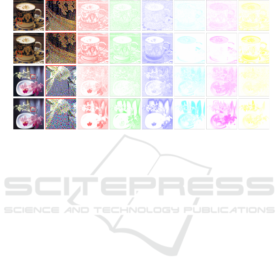
Fig.10 shows an example of our 15-class ED
color halftoning. It is able to create blue-noise dot
distributions for all of the classes (Fig.10(a)-(m),
some empty classes are omitted), as well as their
superimposition (Fig.10(n)). Comparing our result
(Fig.10(o)) with that of the standard ED (Fig.10(p)),
it can be seen that our result demonstrates better blue-
noise property. More CMYK image halftoning results
using our MCED are given in Fig.11.
6.1.2 Comparison with Vector Error-Diffusion
We also compared the performance of our MCED
with the vector error diffusion (VED) (Damera-
Venkata and Evans, 2001) on color image halftoning.
Both algorithms process multiple channels of signals
using ED in a coordinated way. The VED treats the
signals as a vector, and uses an optimum matrix-
valued error filter to introduce the correlation among
the color planes, hence it can generate good color
halftoning results. However, it does not evaluate
the dot distribution on each color planes and the
conflict between them. Thus, the blue-noise property
on each individual color plane cannot be promised.
On the contrary, our MCED can generate blue-noise
outputs on each individual channel of input signal, as
well as their superimposition. Fig.12 demonstrates
a per-channel comparison of the two algorithms on
RGB color image halftoning. It can be seen that our
(a) C
1
(C) (b) C
2
(M) (c) C
3
(Y) (d) C
4
(K)
(e) C
12
(CM) (f) C
13
(CY) (g) C
14
(CK) (h) C
23
(MY)
(i) C
24
(MK) (j) C
123
(CMY) (k) C
124
(CMK) (l) C
234
(MYK)
(m) C
1234
(CMYK) (n) Superimposition (o) Colored (p) Standard ED
Figure 10: CMYK color image halftoning using our 15-
class MCED. Blue-noise dot distributions are generated for
all classes (a)-(m), as well as their superimposition (n).
(o): colored superimposition. (p): halftoning result by the
standard ED. (Best viewed at 100% scaling ratio, 600 DPI).
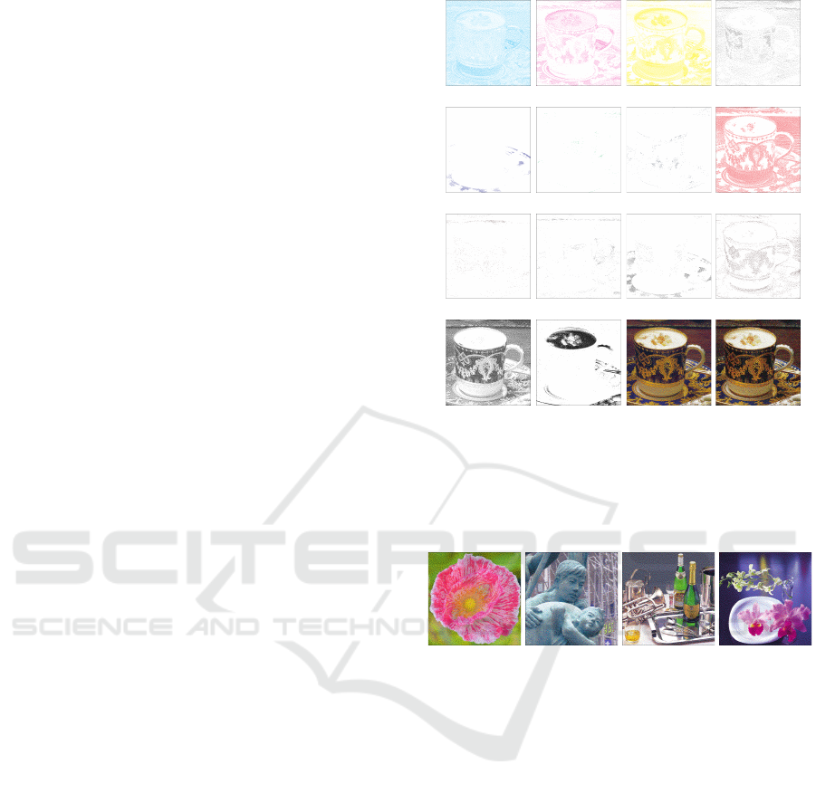
Figure 11: More CMYK color image halftoning results
using MCED. (Best viewed at 100% scaling ratio, 300DPI).
MCED produce obviously better sampling results
with smoother distribution and less artificial textures.
6.2 Multi-tone Error-Diffusion
Multi-toning, also known as multi-level halftoning
(Kang, 1999; Rodrłguez et al., 2008), aims to repro-
duce a continuous tone image with dots of a limited
number of intensities {k
i
|i = 1,··· ,n} (k
i
< k
j
, if i <
j). It is useful in printing with multiple types of inks
or dot sizes. Blue-noise property is also required in
multi-tone images for visually pleasant result, hence
our MCED method is also a solution for multi-tone
image generation.
Given a pixel (x,y) in a continuous tone image
with intensity p(x,y), if k
i
< p(x,y) < k
i+1
, then
p(x,y) can be simulated with a linear combination of
the halftone patterns with intensity k
i
and k
i+1
:
p(x,y) = p
i
(x,y) · k
i
+ p
i+1
(x,y) · k
i+1
, (8)
Multi-Class Error-Diffusion with Blue-noise Property
35
(a) Output (b) Zoom in (c) R (d) G (e) B (f) C (g) M (h) Y
Vector ED
MCED
Vector ED
MCED
Figure 12: Color image halftoning using our MCED method and the Vector ED (Damera-Venkata and Evans, 2001). (a) The
superimposed color halftoning image; (b) Zoom-in viewing of the dot distribution in the red box in (a); (c)-(h) The halftoning
output of the corresponding color plane. (Images best viewed at 100% scaling ratio, 600 DPI).
where p
i
(x,y) and p
i+1
(x,y) are respectively the den-
sities of the halftone pattern of pixels with intensity
k
i
and k
i+1
at (x, y), and p
i
(x,y) + p
i+1
(x,y) = 1. For
j 6= i and j 6= i +1, we let p
j
(x,y) = 0.
Therefore, considering p
i
(x,y) as the input of
class C
i
in a n-class ED, a n-tone image can be
generated by our MCED algorithm. Fig.13 shows an
example of 7-tone image generated with our method.
The halftone patterns for the given intensities {k
i
|i =
1,...,7} can be found in Fig.13(a)-(g), and all of them
possess ideal blue-noise property.
6.3 Color Image Vectorization
A typical catalog of color image vectorization meth-
ods (Swaminarayan and Prasad, 2006) build polygon
meshes on the image plane based on a set of sampling
points. Then, by assigning each polygon node the
image color at the same position, the original image
can be converted to a vector form. The colors inside
a polygon is calculated by interpolating between the
colors of its nodes. Hence, the quality of the sampling
point distribution is crucial for the quality of final
vectorization results.
Our MCED method can provide ideal sampling
point distribution for such a vectorization task. Here,
the input image is in RGB, and the sampling points
can be generated in the three color planes using our
MCED in a similar way as in Section 6.1.1. After
superimposing the sampling points, a planar triangle
mesh is obtained by Delaunay triangulation, which
can be used as the foundation of the vector image.
To preserve the image features during vectoriza-
tion, we extract a salience map from the gradient of
the original color image. At each pixel, the salience
is defined as the sum of the absolute value of the
gradient components, which is calculated by a Sobel
operator. The salience is separately computed in the
three color planes, and the resulting salience map is
also a RGB image. Hence, sampling on the salience
map instead of the original image, we can obtain a
sampling point set that better preserves the features.
7 ANALYSIS AND CONCLUSION
This paper gives an algorithm for multi-class ED.
The key technique of this algorithm is to use the
optimized threshold displacement to minimize the
distortion to the blue-noise property caused by inter-
class correlation in multi-class error-diffusion. Our
experiment shows that this technique can effectively
maintain the blue-noise property that the standard
error-diffusion possesses. The reason for this can be
explained by Fourier transform-based analysis (Knox
and Eschbach, 1993; Gonzalez and Woods, 2001).
7.1 Analysis
According to (Knox and Eschbach, 1993), for the
original ED, the power spectrum B(u,v) of the Fourier
transform of the output image can be written as:
B(u,v) = I(u, v) + F(u, v)E(u,v), (9)
GRAPP 2016 - International Conference on Computer Graphics Theory and Applications
36
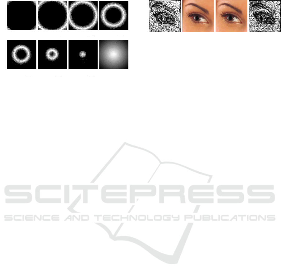
(a) k
1
= 0 (b) k
2
=
43
255
(c) k
3
=
86
255
(d) k
4
=
129
255
(e) k
5
=
172
255
(f) k
6
=
215
255
(g) k
7
=
255
255
(h) M-tone image
Figure 13: An example of 7-tone ED. For an image with
intensity ranges from 1 to 0 (from center to border), a
multi-tone rendering of the image (h) is generated by our
MCED using 7 intensities (tones) given in the figure. (a)-
(g) show the distribution of the pixels with these intensities
respectively. (Images best viewed at 300 DPI).
where I(·) and E(·) are the Fourier transform of the
input image and the error map e(x,y) generated dur-
ing error-diffusion; F(·) is a high-pass filter defined
solely by the diffusion filter.
For each class C
i
, our algorithm is based on (Zhou
and Fang, 2003) by adding an extra modulation m
i
to its threshold, and m
i
includes the displacement t
i
,
which is in nature a noise from other ED classes. Also
according to (Knox and Eschbach, 1993), threshold
modulation is equivalent to sending to the original
ED an equivalent image that is the sum of the original
image and a filtered modulation, where the filter F(·)
is exactly the one in Eq.9. Therefore we have:
B(u,v) = I(u, v) + F(u, v)(D
i
(u,v) + M(u, v))
+F(u,v)E
0
(u,v),
(10)
where D
i
(u,v) is the Fourier transform of d
1i
, M(u,v)
is the Fourier transform of the threshold modulation
r(p) defined in Fig.1 , E
0
(u,v) is the Fourier transform
of the error map e(x, y) for the equivalent image.
Note that t
i
does not appear in Eq.10 because it is a
DC component and is filtered out by F(·). Hence,
threshold displacements do not have influence on the
average density of the output image of any class.
It is also noted that in Eq.10, only D
i
(·) and
E
0
(·) are decided by the threshold displacement {t
i
}.
Considering the fact that t
i
actually has the effect of
decreasing or increasing the amount of slow response
phenomenon at the beginning of the ED, so properly
chosen {t
i
} are able to minimize the amount of
sampling conflict, which in turn can improve the
anisotropy and lower frequency ratio defined in Eq.4.
7.2 Limitation and Future Work
In the experiment results of our paper, smear artifacts
may appear in the sampling classes with low average
(a) (b) (c) (d)
Figure 14: Color image vectorization using our MCED
vs. the standard ED. (a) and (d) are triangulation on
points sampled by Standard ED and MCED, (b) and (c) are
correspong rendering result. The input image is in RGB.
sampling density (Fig.13(g)). This is because we
use s
i
to choose the class with the highest average
intensity when sampling conflict occurs and this may
cause classes with less average intensity to generate
output with lower quality. Hence, the selection of s
i
is a topic to be investigated.
The optimal threshold displacement t
i
= g(p
0
, p
i
)
has the effect of reducing slow response (Haneishi
et al., 1996), which is also called transient effect in
some literature (Zhou and Fang, 2003). That effect
in our MCED is shown obliviously in Fig.14. At
the top of the image, our sampling result (Fig.14(d))
has very weak slow response than that generated by
the standard ED (Fig.14(a)). In fact, the amount of
slow response directly affects the lower frequency
ratio β(p
i
,t
i
) in Eq.4. Our displacement optimiza-
tion automatically guides t
i
to a proper value to
decrease the anisotropy and lower frequency ratio,
and consequently, reduces the slow response. Hence,
introducing threshold displacement into the single-
class standard ED to further reduce its slow response
is also a future research topic to be explored.
REFERENCES
Alliez, P., Meyer, M., and Desbrun, M. (2002). Interactive
geometry remeshing. ACM Trans. Graph., 21:347–
354.
Baqai, F. A., Lee, J.-H., Agar, A. U., and Allebach,
J. P. (2005). Digital color halftoning. IEEE Signal
Processing Magazine, 22:87–96.
Bourguignon, D., Chaine, R., Cani, M.-P., and Drettakis, G.
(2004). Relief: A Modeling by Drawing Tool. In
Eurographics Workshop on Sketch-Based Interfaces
and Modeling (SBM), pages 151–160, Grenoble,
France. Eurographics, Eurographics Association.
Chang, J., Alain, B., and Ostromoukhov, V. (2009).
Structure-aware error diffusion. ACM Trans. Graph.,
28:162:1–162:8.
Damera-Venkata, N. and Evans, B. L. (2001). Design
and analysis of vector color error diffusion halftoning
systems. Image Processing, IEEE Transactions on,
10(10):1552–1565.
Damera-Venkata, N., Evans, B. L., and Monga, V. (2003).
Color error-diffusion halftoning what differentiates
Multi-Class Error-Diffusion with Blue-noise Property
37

it from grayscale error diffusion? IEEE Signal
Processing Magazine, 20:51–58.
Floyd, R. W. and Steinberg, L. (1976). An Adaptive
Algorithm for Spatial Greyscale. Proceedings of the
Society for Information Display, 17(2):75–77.
Gonzalez, R. C. and Woods, R. E. (2001). Digital Image
Processing. Addison-Wesley Longman Publishing
Co., Inc., Boston, MA, USA, 2nd edition.
Haneishi, H., Suzuki, T., Shimoyama, N., and Miyake, Y.
(1996). Color digital halftoning taking colorimetric
color reproduction into account. J. Electronic
Imaging, 5(1):97–106.
Kang, H. R. (1999). Digital Color Halftoning. Society
of Photo-Optical Instrumentation Engineers (SPIE),
Bellingham, WA, USA, 1st edition.
Kim, S. Y., Maciejewski, R., Isenberg, T., Andrews, W. M.,
Chen, W., Sousa, M. C., and Ebert, D. S. (2009).
Stippling by example. In NPAR09, pages 41–50.
ACM.
Knox, K. T. and Eschbach, R. (1993). Threshold
modulation in error diffusion. J. Electronic Imaging,
2(3):185–192.
Li, P. and Allebach, J. P. (2001). Tone-dependent error
diffusion. In Society of Photo-Optical Instrumentation
Engineers (SPIE) Conference Series, volume 4663,
pages 310–321.
Ostromoukhov, V. (2001). A simple and efficient error-
diffusion algorithm. In SIGGRAPH01, pages 567–
572. ACM.
Press, W. H., Teukolsky, S. A., Vetterling, W. T., and
Flannery, B. P. (1992). Numerical Recipes in C: The
Art of Scientific Computing. Cambridge University
Press, New York, NY, USA, 2nd edition.
Rodrłguez, J. B., Arce, G. R., and Lau, D. L. (2008).
Blue-noise multitone dithering. IEEE Transactions on
Image Processing, 17(8):1368–1382.
Swaminarayan, S. and Prasad, L. (2006). Rapid automated
polygonal image decomposition. In Applied Imagery
and Pattern Recognition Workshop, 2006., pages 28–
28. IEEE.
Ulichney, R. A. (1988). Dithering with blue noise.
Proceedings of the IEEE, 76:56–79.
Wei, L.-Y. (2010). Multi-class blue noise sampling. ACM
Transactions on Graphics (TOG), 29(4):79.
Wei, L.-y. (2012). Private communication.
Weissbach, S. and Wyrowski, F. (1992). Error diffusion
procedure: theory and applications in optical signal
processing. Applied Optics, 31:2518–2534.
Zhou, B. and Fang, X. (2003). Improving mid-tone quality
of variable-coefficient error diffusion using threshold
modulation. ACM Trans. Graph., 22(3):437–444.
APPENDIX: Pseudo Code of MCED
Alg.1 is the pseudo-code for the framework of
MCED, and the main functions are explained as
follows:
GetDisplacement() evaluates t
i
by accessing the
lookup table (Fig.6) we described in Section 4.2.
GetCoe f f icient() and GetStandardT hreshold()
are functions for finding appropriate diffusion coef-
ficients and threshold for the standard ED.
Quantize() compares pixel value to the threshold
and returns 0 if below, 1 otherwise. (Eq.1)
HaveCon f lict() returns TRUE if more than one
sampling points from different classes situate at the
current position, and NoCon f lict() indicates only one
class sampled at the position.
FindMaxClass() finds the class whose sum of
densities at all the spatial positions is the maximum.
DistributeError() distributes the quantization er-
rors to neighboring pixels according to the error filter.
Algorithm 1: Multi-Class Error-Diffusion.
1: for each spatial position (x,y) do
2: p
0
(x,y) ←
n
∑
i=1
p
i
(x,y)
3:
4: for each spatial position (x,y) do
5: // The first step Q
i
6: for each class i := 0 to n do
7: t
i
(x,y) ← GetDisplacement(p
0
(x,y), p
i
(x,y))
8: a
(i)
jk
← GetCoe f f icient(p
i
(x,y))
9: u
i
(x,y) ← GetStandardT hreshold(p
i
(x,y))
10: u
i
(x,y) ← u
i
(x,y) + t
i
(x,y)
11: for each class i := 0 to n do
12: c
0
i
← Q(p
i
(x,y) + b
i
(x,y),u
i
(x,y)) // Eq.1
13:
14: // The second step E
i
15: if c
0
0
(x,y) = 1 then
16: if HaveCon f lict() then // i.e.:
∑
i6=0
c
0
i
> 1
17: c
0
(x,y) ← 1
18: e
0
(x,y) ← p
0
(x,y) − c
0
(x,y)
19: minclass ← FindMaxClass()
20: for each class i := 1 to n do
21: if i = minclass then // i.e.:s
i
= TRU E
22: c
i
(x,y) ← 1
23: else
24: c
i
(x,y) ← 0
25: e
i
(x,y) ← p
i
(x,y) − c
i
(x,y)
26: else if NoCon f lict() then // i.e.:
∑
i6=0
c
0
i
= 1
27: for each class i := 0 to n do
28: c
i
(x,y) ← c
0
i
29: e
i
(x,y) ← p
i
(x,y) − c
i
(x,y)
30: else // No class sampled:
∑
i6=0
c
0
i
= 0
31: for each class i := 0 to n do
32: c
i
(x,y) ← 0
33: e
i
(x,y) ← p
i
(x,y) − c
i
(x,y)
34: else // When c
0
0
= 0
35: for each class i := 0 to n do
36: c
i
(x,y) ← 0
37: e
i
(x,y) ← p
i
(x,y) − c
i
(x,y)
38:
39: for each class i := 0 to n do
40: DistributeError(i,x,y,e
i
(x,y),a
(i)
jk
)
GRAPP 2016 - International Conference on Computer Graphics Theory and Applications
38
