Content based Computational Chromatic Adaptation

Fatma Kerouh

1,2

, Djemel Ziou

and Nabil Lahmar

Institute of Electrical and Electronic Engineering, M’Hamed BOUGARA University, Boumerdes, Algeria

USTHB, Image Processing and Radiation Laboratory, Algiers, Algeria

epartement d’Informatique, Universit

e de Sherbrooke, Sherbrooke, Qc., J1K 2R1, Canada

Keywords:

Computational Chromatic Adaptation, von Kries Transform, Bradford Transform, Sharp Transform, Spatial

Content.

Abstract:

Chromatic adaptation is needed to accurately reproduce the color appearance of an image. Imaging systems

have to apply a transform to convert a color of an image captured under an input illuminant to another output

illuminant. This transform is called Chromatic Adaptation Transform (CAT). Different CATs have been pro-

posed in the literature such as von Kries, Bradford and Sharp. Both these transforms consider the adjustment

of all the image spatial contents (edges, texture and homogeneous area) in the same way. Our intuition is that,

CATs behave differently on the image spatial content. To verify that, we prospect to study the well known

CATs effect on the image spatial content, according to some objective criteria. Based on observations we

made, a new CAT is derived considering the image spatial content. To achieve that, suitable requirements for

CAT are revised and re-written in a variational formalism. Encouraging results are obtained while comparing

the proposed CAT to some known ones.

1 INTRODUCTION

The Human Visual System (HVS) has the partic-

ularity of dynamically adapting to the changing

of light conditions. In fact, HVS is able to carry

out automatically a chromatic adaptation in order

to preserve color constancy. However, imaging

systems as scanners and digital camera have not

the ability to adjust their sensors relative response

as the HVS. In this case, a transform is needed. It

is called Chromatic Adaptation Transform (CAT).

Computational color adaptation refers to the use of

algorithms to predict the real color of an object when

it is seen and captured under different light sources.

It is a basic operation in the color appearance model

(Fairchild, 2005) (Madin and Ziou, 2014), where

the goal is to provide complete and faithful color

information that fulﬁls the requirements of real

world applications including, white balance (Wilkie

and Weidlich, 2009), (Laine and Saarelma, 2000),

(Lee and Goodwin, 1997), (Hirakawa and Parks,

2005), (Spitzer and Semo, 2002), color reproduction

(Fairchild, 2005), and color based skin recognition

(Bourbakis et al., 2007). Assuming the light sources

known, a deterministic prediction is possible if the

image formation model allows to write an output

image as a function of an input image. According

to the von Kries chromatic adaptation theory (Kries,

1970), a color prediction of an object is reached by

independently scaling each sensor output value by

the output to input ratio in the RGB color space. The

implementation is straightforward. The output image

is obtained by multiplying the input image and the

diagonal matrix of ratios









= M

−1





α 0 0

0 β 0

0 0 γ













(1)

A linear CAT can be written as M

−1

DM, (equation

(1)), where M is a matrix related to the used color

space and D stands for the von Kries transform. Any

CAT can be seen as a linear transform of a color space

to another one of the same dimension. Where, the

columns of M are the basis of the color space and D

is a diagonal matrix specifying colors dispersion ac-

cording to each element of the basis. Given the input

color space and the von Kries transform, another is-

sue concerns the choice of the output color space. In

some previous works, the space is obtained experi-

mentally by color matching paradigms where the cri-

teria to choose the color space are implicit. However,

Kerouh, F., Ziou, D. and Lahmar, N.

Content based Computational Chromatic Adaptation.

DOI: 10.5220/0005678100390047

In Proceedings of the 11th Joint Conference on Computer Vision, Imaging and Computer Graphics Theory and Applications (VISIGRAPP 2016) - Volume 2: IVAPP, pages 41-49

ISBN: 978-989-758-175-5

some criteria were established. According to Lam

(Lam, 1985), the CAT should maintain constancy for

all neutrals, work with different adapting illuminant,

and it should be reversible. More theoretical studies

were conducted to identify the requirements to select

the suitable color space for color prediction (Gortler

et al., 2007; West and Brill., 1982). Among these

requirements, narrowing the sensor spectral sensitiv-

ity leads to more accurate color prediction. Based

on these ﬁndings, Finlayson et al proposed the Sharp

transform (Finlayson et al., 1994). A quantitative

evaluation and comparison between some existing

transforms can be found in (Luo, 2000; Holm et al.,

2010; Bianco and Schettini, 2010). According to

these evaluations, the Bradford, Bartleson, Sharp, and

CMCCAT2000 transforms perform better than many

others. Note that the experimental data set used to

derive the transform is another issue. The available

data sets are chosen according to some protocols and

viewing conditions to reﬂect realistic situations (Luo,

2000). However, the image content effect on color

prediction is not understood because in most previ-

ous works the whole data are transformed into XY Z

color space coordinates and used to derive a CAT. To

summarize, four research area can be discussed in the

color adaptation ﬁeld. The ﬁrst one concerns the best

color space used to implement a CAT. The second is-

sue is about the used transform to adapt the image

color appearance. The third one refers to the choice

of the best output color space and the last research

area concerns the experimental datasets. The purpose

of this work falls under the second research area. Our

aim is to propose a new color adaptation transform

that fulﬁls some particular requirements.

The image content refers to spatial information

such as edges and textures at low abstraction level

and to events such as objects, their relationships and

context at high abstraction level. For example, the

color prediction at a pixel is independent from the

color of the other pixels. Ignoring spatial correlation,

the transform accuracy can be high in some areas of

an image and low in others. In this paper, we em-

pirically studied the inﬂuence of CATs on the low

level image content (which we call the spatial con-

tent) that are colors, edges, textures and homogeneous

areas. Based on conclusions we made and inspired

by the Sharp transform proposed earlier by Finlayson

et al.(Finlayson et al., 1994), we propose new con-

straints and formulate the derivation of CAT as a vari-

ational problem. The resulting transform is compared

to some existing transforms based on the von Kries

theory. The next section is devoted to studying the

CATs inﬂuence on image spatial information. In Sec-

tion 3, we present a new proposed approach to derive

a CAT. Experimental results are addressed in Section

4. The last section concludes this work with some

valuable issues.

2 COMPUTATIONAL

CHROMATIC ADAPTATION

EFFECT ON THE IMAGE

CONTENT

In this section, a series of tests are conducted allowing

to understand the von Kries-based CATs effect on im-

ages spatial content. In our experiments, we pay par-

ticular attention to edges, texture and homogeneous

areas. Texture is characterized by its form, coarse-

ness and complexity while edges are characterized by

their sharpness and orientation.

2.1 Test Data

The reliability of experiments on chromatic adapta-

tion depends on the test data accuracy. In our experi-

ments, the used images are built using the image for-

mation model. For a surface with a reﬂectance func-

tion R(λ) and an illuminant E(λ), the discrete image

formation model is given by:

X = C

700

∑

λ=400

E(λ)R(λ)VW X(λ) (2)

Y = C

700

∑

λ=400

E(λ)R(λ)VWY(λ) (3)

Z = C

700

∑

λ=400

E(λ)R(λ)VW Z(λ). (4)

Where,

• VW X , VWY and VWZ are considered as the VW

sensor sensitivities (Finlayson et al., 1994).

• Reﬂectance images R, are taken from the G. Fin-

layson et al. collection (Finlayson et al., 2004).

This collection consists of a set of reﬂectance im-

ages of everyday objects with high spatial and

spectral resolutions.

• The incandescent illuminant A and daylight D65,

which are experimental illuminant approved by

the CIE (CEI, 1998), are used.

• The constant C = 100

∑

700

λ=400

E(λ)VWY (λ) is

used for normalization, yielding a value of Y =

100 for a perfect diffuser, which means that the re-

ﬂectance is equal to one for all wavelengths (Lee

and Goodwin, 1997). The wavelengths are sam-

pled by an increment of 10nm in the visible inter-

val [400,700]nm.

IVAPP 2016 - International Conference on Information Visualization Theory and Applications

• Finally, to display the image, the sRGB space is

used. This color space is proposed by Hewlett-

Packard and Microsoft via the International Color

Consortium ICC (Stokes et al., 1996).

Having the reﬂectance multispectral images R, vari-

ous test images could be constructed, according to the

image formation model, using different light sources

E and VW sensors sensitivity.

2.2 Methodology

The aim now is to study the CATs effect on the image

content (homogeneous area, edges and texture). To

achieve that, the following steps are followed.

• Twenty-three reﬂectance images of various ob-

jects and two standard illuminant (illuminant

”D65” and illuminant ”A”) are used to construct

test images using the image formation model as

explained before. Altogether, there are 46 test

images categorized in groups, which we will call

groupA and groupD65.

• Consider a pair of images of the same scene

taken under the standard illuminant ”D65” and

”A”. The aim is to transform the test image un-

der ”D65” to the estimated image under ”A” by

using the von Kries based CATs. According to

our experimentation, we found that the Bradford

transform (CAT

) provides the smallest distortion

of the estimated images. Consequently, in the

remainder of this section we will present only

the scores of CAT

. Hence, a third set of im-

ages, groupD65A, is built from groupD65 by us-

ing CAT

• To evaluate distortions on step edge pixels, we

consider the edge magnitude and orientation. For

this purpose, we compute the mean ν, the vari-

ance σ

and the phase θ of the gradient images as

follows:

ν =

N × M

∑

|||G(i, j)|| − ||G

re f

(i, j)||| (5)

N × M

∑

(|||G(i, j)||−||G

re f

(i, j)|||−ν)

(6)

θ = arccos

G · G

re f

kGkkG

re f

(7)

where G and G

re f

are the gradient vectors of the

estimated and reference N × M images, respec-

tively and · is the dot product. Note that, the gra-

dient is estimated by using the ﬁrst partial deriva-

tives of Gaussian.

• To assess the CAT

effect on texture, a quanti-

tative evaluation requires to use texture descrip-

tors that allow measuring deformation. For this

purpose, we use nine descriptors estimated from

four cooccurrence matrices, corresponding to dis-

placements equal to one in directions 0, π/4, π/3,

and 3π/2. The computation rules for these de-

scriptors can be found in (Haralick et al., 1973).

The squared Euclidean distance between the tex-

ture descriptors of the estimated and reference im-

ages is used to measure the CAT

effect.

• To quantify the distortion between the adapted

and the reference image, S-CIELAB error pre-

diction metric is considered. However, for com-

plex scenes, it should be noted that the varia-

tion of CIELAB ∆E

is greater than the variation

of S-CIELAB ∆E

(Aldaba et al., 2006), but the

shape of both variations is similar. Hence, we pro-

pose to use the color difference formula CIELAB

∆E

between the adapted and the reference im-

age. The ∆E

between two colors (L

)

and (L

) is computed as follows (Green and

MacDonald, 2002):

∆E



∆L





∆C





∆H



(8)

Where ∆L = L

− L

stands for the luminosity,

∆C = C

− C

the chroma and ∆H = {(∆a)

(∆b)

− (∆C)

}

the hue.

+ b

, C

+ b

, ∆a = a

− a

∆b = b

− b

, k

= 1, S

= 1 + 0.045C,

= 1 + 0.015C, k

= k

= 1.

Note that, a ∆E

of 1.0 is the smallest color dif-

ference that the human eye can notice.

2.3 Experimental Results

For the quantitative evaluation of the adapted images,

∆E

color difference is computed between original

and adapted images by considering, all pixels, ho-

mogeneous area and edge pixels. Note that, for the

caused distortion to both texture and edge areas, grey

level images have been considered. Table 1 shows

the mean of ∆E

according to the image content. We

can notice that, the metric value changes according

to the image content; it is not the same for edge pix-

els, homogeneous areas and overall the image pixels.

In fact, compared to all pixels, the estimated error

from homogeneous area and edges is about 7% and

3% greater, respectively. Thus we conclude that, the

chromatic adaptation inﬂuence depends on the image

spatial content.

Content based Computational Chromatic Adaptation

Table 1: Mean of ∆E

metric for CAT

Bd f

as a function of

image content.

Image content ∆E

All pixels of the image 1.487

Edge pixels 1.535

Homogeneous area pixels 1.589

Our purpose now is to detect which speciﬁc char-

acteristics are affected in texture and edges (strength

or orientation or both). For that, as explained in the

methodology sub-section, separate deformation mea-

surement was deﬁned for each image content. Table 2

presents the absolute difference in gradient magnitude

of the two groups of images, groupA and groupD65A,

according to a certain threshold, which is a percent-

age of the maximum value of the gradient magnitude.

Thus a threshold of 5% corresponds to 5% of the max-

imum value of the gradient magnitude in the differ-

ence image. We noticed that, for a threshold (Th)

of 5, 27.473% of all the edge pixels provides a mean

value of 1.183 and a variance value of 0.788; this is

not negligible relatively to the min and the max val-

ues of gradient magnitude, which are 0.454 and 9.078,

respectively. Furthermore, for a threshold of 10, the

percentage of eligible edge pixels is 14.084%, with

a mean value of 1.687 and the associated variance is

1, which is also signiﬁcant. Based on the obtained

values, we can notice that the mean and the variance

values increase with the threshold, while the percent-

age of eligible edge pixels decreases. Thus, the chro-

matic adaptation transformation produces an image

with less contrast than the reference image, since the

difference in image edges is not negligible. As con-

clusion, edge strength is modiﬁed while applying a

CAT.

Table 3 shows the mean and variance of the angle

between the gradient vector of the two groups of im-

ages, according to a certain threshold T h. We notice

a considerable deviation in the gradient. In fact, from

the threshold 5 to 25, the mean of the deviation ranges

from 9.9 to 6.13 degrees. This is signiﬁcant consider-

ing the percentage of eligible gradient vectors which

are between 36.85% and 6.85%. To summarize:

• While increasing the threshold value, both the

mean and the variance of the absolute difference

in magnitude of gradients increase. However, the

percentage of eligible edge pixels decreases.

• The mean over the smallest and highest gradient

magnitudes ratios show that, the CAT

effect is

stronger for details than it is for obvious edges.

• Both the mean error and variance of edge orien-

tation decrease when the smallest gradient magni-

tude increases. Again, details are the most vulner-

able.

Table 2: Mean and variance of in gradient magnitude of the

two image groups, according to empirical threshold.

T h ν σ

Max grad Min grad % of edge

pixels

5% 1.183 0.788 9.078 0.454 27.47

10% 1.687 1.000 9.078 0.908 14.08

15% 2.215 1.313 9.078 1.362 7.362

20% 2.875 1.773 9.078 1.816 3.644

25% 3.592 2.084 9.078 2.270 1.998

Table 3: Mean and variance of gradient angle between gra-

dient vectors of the two image groups, according to empiri-

cal threshold.

T h ν σ

% of edge pixels

5% 9.90 0.23 36.85

10% 8.62 0.20 22.43

15% 7.54 0.25 14.64

20% 6.63 0.19 10.15

25% 6.13 0.17 6.85

Table 4: Texture characteristics for displacement equal to 1

in the direction 0

◦

Features Ref Ad Euclidean distance

Mean 15.248 14.762 0.486

Variance 52.115 50.544 1.571

Energy 0.031 0.030 0.001

Entropy 4.138 4.140 0.001

Contrast 2.086 2.238 0.152

Homogeneity 0.779 0.775 0.004

Correlation 51.073 49.426 1.647

Cluster Shade 1137.740 954.656 183.080

Cluster Prominence 73821.300 66636.700 7184.660

Obtained texture features using groupA and

groupD65A image sets are tabulated on Table 4. The

Euclidean distance is used to perform a one-to-one

comparison of these characteristics computed on a

reference image (Ref) and an adapted one (Ad). No-

tice that, the two features that undergo a signiﬁcant

change are the shade and the prominence. The vari-

ation in cluster shade implies that the image loses its

symmetry. While change in prominence means that,

the number of pixels having grey levels close to the

mean changes.

To conclude, CAT

depends on the image spa-

tial content. Indeed, homogeneous areas colors are

more distorted than edge areas colors. The orienta-

tion and magnitude of weak edges are more distorted

than those of obvious edges. For texture, the shade

and prominence are the most deformed. Hence, our

aim in the next section is to propose a new CAT tak-

ing the image spatial contents into consideration.

IVAPP 2016 - International Conference on Information Visualization Theory and Applications

3 SPATIAL COMPUTATIONAL

CHROMATIC ADAPTATION

An image can be seen as the summation of several

cues such as shading, shadow, blur, edges and tex-

tures originating from physical phenomena which are

illumination, reﬂectance and sensor sensitivity. Based

on observations we made in the previous section, we

can reasonably assume that, the cues behave differ-

ently when a CAT is applied. One can derive a CAT

for each cue. For example, a step edge CAT can be

estimated and used to transform pixels having a high

gradient magnitude. To estimate a CAT, we propose

to revisit the variational formulation of Finlayson et

al. (Finlayson et al., 1994) and include the image data

d(λ) in the new CAT constraints. In addition, the CAT

must fulﬁl the following requirements:

• Preserving the sensor gamut: This requirement

allows the preservation of the sensed set of col-

ors. Reducing this set, implies a reinforcement of

metamerism. Increasing it may lead to output col-

ors that are not physically realizable on the sensor.

• Reducing the overlap between spectral sensitiv-

ity of colored sensors: As showed in (Finlayson

et al., 1994), this requirement allows a better color

constancy. It can be formalized as a sharpening

problem of sensors spectral sensitivities. Unlike

the formalism of Finlayson et al., the sharpening

of one sensor sensitivity function is related to the

sharpening of the other sensitivity functions of the

same sensor.

• Having a positive sensor response to a given data:

It has been shown that this constraint leads to

more accurate CAT (Drew and Finlayson, 2000).

• Being insensitive to noise: Noise insensitivity is

beneﬁcial, especially, when the CAT is estimated

from real samples that can be noisy. We wish that,

the transform remains unchanged when changing

the variance of a white noise image. However, the

energy of a spectral sensitivity function increases

with the white noise variance because it is equal

to the variance of its response to the centred white

noise. Consequently, the last requirement can be

fulﬁlled by setting the energy of sensitivity func-

tions to a constant.

More formally, we denote the original sensor sen-

sitivity functions as {b

(λ)}

k=1

. The sharpening of

this sensor through a linear transform provides new

sensitivity functions noted c

(λ) = β

B(λ)

, where

B(λ) is the original sensor sensitivity functions vec-

tor and β is the linear sharpening transform. In what

follows, we will show how to estimate the sharpening

transform in the case of the k

sensitivity function.

The same procedure is applied for the two other sen-

sitivity functions. The response of the k

sharpened

sensitivity function to the data d(λ) is given by:

d(λ)c

(λ) = d(λ)B(λ)

= D(λ)

where β

is the vector of sharpening coefﬁcients. Let

Γ be the entire visible interval; Γ = Ω

∪Φ

, where Φ

is the sharpening interval associated with the k

sen-

sitivity function. The above mentioned requirements

are translated to:

• Preserving the new sensor Gamut by minimizing

the difference between the responses to the input

data of the original and the new sensitivity func-

tion, that is:

min

(D(λ)

− d(λ)b

(λ))

dλ

• Reducing the overlap between spectral sensitivi-

ties by minimizing the contribution of the other

spectral sensitivities within the sharpening inter-

val Φ

, that is:

min

∑

j6=k

(λ)

)

dλ and minimizing the

spectral response outside the sharpening interval,

that is:

min

Ω

(D(λ)

)

dλ

• Reaching a positive solution when

min

B(λ)

≥ 0, ∀λ ∈ Γ

• Setting the ﬁlter energy to one ensuring a robust-

ness of the sharpening transform to the additive

white noise:

Ω

(B(λ)

)

dλ = 1

We will write the discrete version of the variational

problem used to ﬁnd the optimal β

. The combination

of the ﬁrst, the second and the fourth requirement into

a variational formulation by additive rule is straight-

forward. However, the positivity constraint is not in

an integral form. We propose to use an interior point

formulation, where a logarithm slack function ensur-

ing positivity is used, (Forsgren et al., 2002). Let

us assume that we have N images (or image areas)

taken under different illuminant. We consider ρ and

µ Lagrange multipliers and ε > 0 a barrier parameter

of the slack variables r

(λ), assumed positive. More-

over, the importance of each of the above measures is

not deﬁned. One can use a weighted combination of

these measures and estimate the weights. However,

the number of unknowns increases and the estimation

may be under conditioned. We then propose to use

binary weights allowing to identify the relevance of

each measure. Given the color triplets {d

}

n=1

and

B(λ), the sharpening transform is estimated by mini-

mizing the following objective function:

Content based Computational Chromatic Adaptation

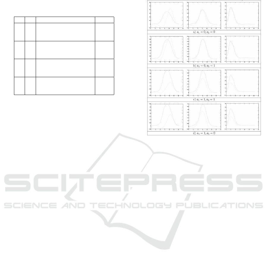
Table 5: The four transfer matrices obtained with the image

content-based method.

Matrix CAT

1 1 1.1160 −0.045 −0.071 CAT

d11

−0.568 1.3970 0.1710

0.0290 0.0800 0.8910

0 1 1.1260 −0.060 −0.066 CAT

d01

−1.074 1.8470 0.2270

0.0180 0.0820 0.9000

1 0 2.0250 −1.092 0.0670 CAT

d10

−1.716 2.8450 −0.128

0.0440 −0.189 1.1450

0 0 2.1590 −1.206 0.0470 CAT

d00

−1.094 2.1610 0.0670

0.0270 −0.201 1.1740

(β,µ) = a

∑

n=1

∑

i∈Φ

(λ

)

−

(λ

))

δλ +

∑

n=1

∑

i∈Φ

∑

j6=k

(λ

)

δλ +

∑

n=1

∑

i∈Ω

(λ

)

δλ +

ρ(

∑

i∈Γ

(B(λ

)

δλ − 1) +

∑

i∈Γ

(B(λ

)

− r

(λ

))δλ − (9)

∑

i∈Γ

log(r

(λ

))δλ

where D

(λ) = d

(λ)B(λ) and a

anda

are the

weighting parameters that have been added to select

the best requirements. The above equations are solved

by using the Newton method to determine β

, the La-

grange multipliers µ, ρ, and ε as well as the slack

function r

(λ). Note that, the earlier formulation pro-

vided by Finlayson et al. can be obtained by setting

= a

= 0, ρ = 1, ε = 0, µ = 0, and d

(λ) = 1. The

formulation with the positivity constraint described

in (Drew and Finlayson, 2000) can be obtained by set-

ting a

= a

= 0, ρ = 1 and d

(λ) = 1. In addition, the

transformation of an image under illuminant a to an

other illuminant b is given by β

−1

a,b

β, where D

a,b

the von Kries diagonal matrix, and β is the sharpening

matrix where the columns are {β

}

k=1

. By resolving

the above equation, four transformation matrices are

obtained by combining coefﬁcients a

and a

which

may be 0 or 1 (Table 5).

Figure 1A depicts the VW sensors and the four

new sensors, obtained by combining both coefﬁcients

and a

. Note that, the combination a

= a

= 0

corresponds to the sharp transform of Finlayson et al.

According to this ﬁgure, two cases are distinguish-

Figure 1: The new sensors in dotted lines compared to the

VW sensor in solid line for each transfer matrix obtained by

the proposed approach.

able, depending on whether coefﬁcient a

is 0 or 1.

In the ﬁrst case (i.e., a

= 0), the resulting sensors are

narrower and have greater amplitudes compared to the

VW sensor. In the second case, in contrast, the sen-

sors are larger and their amplitude is smaller than that

of the VW sensor. Another signiﬁcant remark relates

to the negative values of the spectral distributions of

the sharpened sensors, which are due to negative val-

ues of the calculated transfer matrices. This can cause

color saturation problems during the imaging process.

4 EXPERIMENTAL RESULTS

In this section, we aim to evaluate the four proposed

chromatic adaptation transforms performance. First,

we start by producing test images under illuminants

A and D65. Example of test images are depicted

in ﬁgures 2 and 3. Then, we change the illumi-

nant of images under D65 toward illuminant A us-

ing various CAT s (proposed and existing). The com-

parison is carried out between test images generated

using the image formation model under illuminant A

(ground truth) and the adapted ones using different

CAT s. This comparison is achieved following two

evaluation criteria. The ﬁrst one is related to the per-

ceptual degradation assessment using the color differ-

ence metric presented earlier called ∆E

. The second

one is intended to measure the CAT

s effect on the im-

age contents deﬁned by edges and texture properties.

IVAPP 2016 - International Conference on Information Visualization Theory and Applications

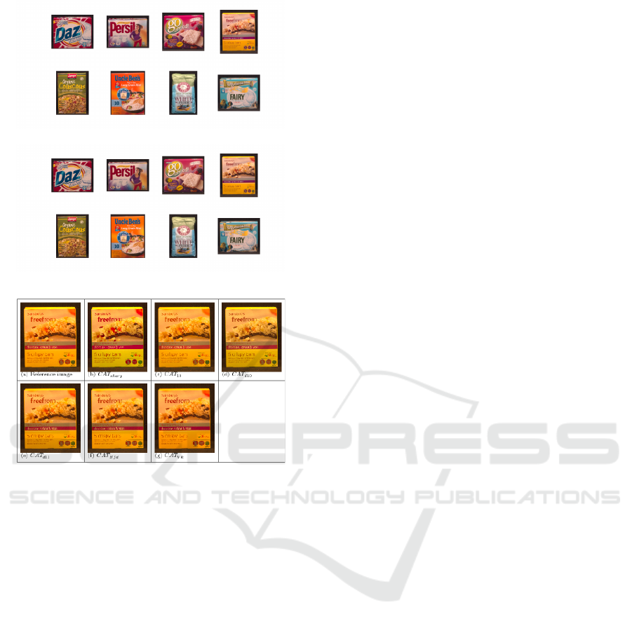
Figure 2: Examples of test images under illuminant D65.

Figure 3: Examples of test images under illuminant A.

Figure 4: ”Freeform” images obtained with the different

CAT transforms, under illuminant A.

Figure 4, illustrates one example of corresponding

images obtained by various CAT s on Freeform image.

4.1 Colorimetric Evaluation

CIE∆E

color difference is used, in Lab space, to

estimate the perceptual color difference between the

ground truth and the adapted image. It calculates an

ellipsoid tolerance around the target color, such that

the color belonging to this ellipsoid will be considered

identical. This metric is recommended by CIE for the

color difference quantiﬁcation. Computed ∆E

obtained images illustrated in Figure 4 are tabulated

on Table 6. We can notice that, the transformations

CAT Brad f ord( CAT

), CAT

d11

, CAT

d10

in that order

provide the best results in terms of perception. How-

ever, the CAT Sharp(CAT

) quantitative evaluation is

less acceptable. From ∆E

metric stand of point, a

∆E

value less than or equal to four is considered to

be satisfactory (CEI, 2004).

Thus we conclude that, the proposed image content

based transform CAT

C11

provides more accurate per-

formance compared to both CATVonKries(C AT

) and

CAT

. Furthermore, a competitive performance are

noticed against CAT

4.2 Content-based Evaluation

This evaluation involves calculating some charac-

teristics related to the image content (edges and

texture area) as explained previously. The considered

characteristics are computed on the adapted images

using the proposed CATs and the considered existing

ones (Sharp, Von Kries and Bradford transforms).

Then, the error is quantiﬁed using some speciﬁc

criteria.

Edge Evaluation

We compute the edge map of the adapted and the

ground truth images. The comparison concerns edges

strength and orientation, as explained previously. Ta-

bles 7, 8 and 9 present the mean and the variance

of the absolute difference between the gradient mag-

nitude of the adapted and the reference images, for

each transformation. Each table is related to a given

threshold. This threshold stands for the percentage of

a gradient magnitudes maximum. It is especially used

to assess the signiﬁcance of the gradient magnitude

difference, which can be manifested as a difference in

contrast between two image groups. Table 7 presents

the obtained results for a threshold of 5% of the max-

imum value of the gradient magnitude difference in

images. It can be seen that, the CAT

transform per-

forms better than the other transformations in terms

of mean values. We note that, Compared to CAT

, the

CAT

d11

transform obtains very close results in terms

of mean value and performs better in terms of vari-

ance value and maximum magnitude value. Concern-

ing Tables 8 and 9 which list the results for larger

thresholds, namely 15% and 25%, the CAT

d11

trans-

form obtains the best results in term of mean, variance

and maximum value. All in all, the proposed content-

based transform performs slightly better than the oth-

ers in preserving image edges.

Table 10 shows the mean and the variance values

of the angle between the gradient vectors of the two

image groups for each transformation. The CAT

d11

gradient vector deviation is about 3.431 degrees com-

pared to 6.551 and 8.68 degrees for CAT

and CAT

respectively. According to these results we can argue

that, the proposed CAT

d11

provides the best perfor-

mance in terms of edge pixels orientation preserva-

tion.

Texture Evaluation

We compare the texture descriptors of the reference

and the adapted images as explained in the previous

section. Table 11, shows the Euclidean distance of

Content based Computational Chromatic Adaptation

Table 6: Computed color error on images of Figure 4.

CAT

d10

CAT

d11

∆E

1.487 2.285 6.377 2.438 2.080 1.92

Table 7: Mean and variance of the absolute difference

in gradient magnitude between the ground truth and the

adapted images for threshold equal to 5%.

ν σ

Max grad Min grad % of edges pixels

CAT

6.160 21.427 40.083 2.004 23.52

CAT

d01

1.978 2.242 12.347 0.617 35.28

CAT

d10

1.449 1.585 10.085 0.504 23.99

CAT

d11

1.148 0.673 8.989 0.449 29.77

CAT

1.804 1.590 11.583 0.579 28.76

CAT

1.183 0.788 9.078 0.454 27.47

Table 8: Mean and variance of the absolute difference

in gradient magnitude between the ground truth and the

adapted images for a threshold of 15%.

ν σ

Max grad Min grad % of edges pixels

CAT

11.222 21.152 40.083 6.013 8.07

CAT

d01

3.362 2.500 12.644 1.897 14.52

CAT

d10

3.940 3.3860 13.254 1.988 15.26

CAT

d11

2.072 1.054 8.988 1.349 9.53

CAT

3.070 1.483 11.583 0.738 10.82

CAT

2.215 1.313 9.078 0.362 7.362

the texture features, for each transformation matrix.

An ordered ranking of the transformations accord-

ing to the number of texture features where they per-

form, provides (in descending order): CAT

d11

, CAT

CAT

d10

, CAT

d01

, CAT

and CAT

. Thus, CAT

d11

more accurate in terms of texture mean, contrast,

homogeneity. Especially, cluster shade and cluster

prominence which are the most affected texture prop-

erties according to the previous section. That means

that, these properties are better preserved by the pro-

posed CAT

d11

5 CONCLUSION

This paper presents a new chromatic adaptation trans-

forms transform (CAT ) by considering the content in-

formation of a given image. Two main contributions

are proposed. First, the authors prove that the chro-

matic adaptation transform affects differently the im-

age contents, especially edges and texture area which

are two essential elements in the human visual sys-

tem. Second, the authors propose a new reformu-

lation of chromatic adaptation transform (CAT) that

considers the image content information. To achieve

the ﬁrst purpose, some well knowns CAT s are con-

sidered. According to a perceptual color difference

metric, results prove that these transforms depend

on the image spatial content. Indeed, the homoge-

neous area colors are more distorted than those of

edge areas. Furthermore, edge orientation and mag-

nitude of weak edges are more distorted than those

of obvious edges. For texture, the shade and promi-

Table 9: Mean and variance of the absolute difference

in gradient magnitude between the ground truth and the

adapted images for a threshold of 25%.

ν σ

Max grad Min grad % of edges pixels

CAT

13.249 18.226 40.083 8.017 5.47

CAT

d01

3.982 2.690 12.644 2.529 9.5

CAT

d10

4.665 3.839 13.254 2.651 10.58

CAT

d11

2.689 1.618 8.988 2.247 4.31

CAT

3.658 1.320 11.583 2.317 6.96

CAT

2.875 1.773 9.078 2.27 3.64

Table 10: Mean and variance of absolute difference in gra-

dient angle between the the ground truth and the adapted

images for a threshold of 5%.

ν σ

% of edge pixels

CAT

8.680 0.685 23.52

CAT

d01

5.574 0.197 35.28

CAT

d10

5.913 0.268 23.99

CAT

d11

3.431 0.160 29.77

CAT

7.249 0.365 28.76

CAT

6.551 0.384 27.47

Table 11: The Euclidean distance of texture features for

each CAT .

Features CAT

CAT

d01

CAT

d10

CAT

d11

CAT

Mean 0.336 0.283 0.152 0.070 0.174 0.486

Variance 5.993 0.687 0.592 0.462 0.308 1.571

Energy 0.002 0.001 0.001 0.001 0.001 0.001

Entropy 0.107 0.011 0.042 0.006 0.011 0.001

Contrast 0.213 0.106 0.027 0.071 0.072 0.152

Homogeneity 0.022 0.004 0.006 0.000 0.002 0.004

Correlation 5.384 0.740 0.605 0.426 0.343 1.647

Shade 279.2 112.6 77.8 59.61 68.35 183.0

Prominence 10330 4044 2825 900.5 2526 7184

nence features are the most deformed features. Based

on these conclusions, the authors reformulate the

sharp transform considering new CAT

s requirements.

From the variational formulation, four transforms

have been proposed. Their performances are quan-

titatively evaluated against some well known trans-

forms (Sharp, Bradford and von Kries). Experimental

results showed that one of these transforms, namely

CAT

d11

, preserves better edges and texture features

than the considered existing CAT s. Thus, taking the

image content into account, to derive CAT s, can im-

prove the preservation of both the color and the spa-

tial content of the adapted images. Future works will

involve the consideration of a large database and es-

pecially noisy data. In addition, the authors prospect

to use other evaluation criteria.

REFERENCES

Aldaba, M. A., Linhares, J. M., Pinto, P. D., Nascimento,

S. M., and K. Amano, D. H. F. (2006). Visual sensi-

tivity to color errors in images of natural scenes. In

Visual Neuroscience, 23:555-559.

Bianco, S. and Schettini, R. (2010). Two new von kries

based chromatic adaptation transforms found by nu-

IVAPP 2016 - International Conference on Information Visualization Theory and Applications

merical optimization. In Color Research and Applica-

tion, 35(3):184-192,.

Bourbakis, N., Kakumanu, P., Makrogiannis, S., Bryll, R.,

and Panchanathan, S. (2007). Neural network ap-

proach for image chromatic adaptation for skin color

detection. In Int. Journal of Neural Systems, 17(1):1-

12.

CEI (1998). Commission internationale de l’eclairage.

interim colour appearance model (simple version,

ciecam97s). In Technical Report, 131.

CEI (2004). Commission internationale de l’eclairage. a

review of chromatic adaptation transforms. technical

report, 160. In Visual Neuroscience.

Drew, M. S. and Finlayson, G. (2000). Spectral sharpening

with positivity. In J. Opt. Soc. Am. A, 17:1361-1370,.

Fairchild, M. D. (2005). Color appearance models. In Sec-

ond Edition, Wiley.

Finlayson, G., Drew, M., and Funt, B. (1994). Spec-

tral sharpening: Sensor transformations for improved

color constancy. In J. Opt. Soc. Am. A, 11(5):1553-

1563.

Finlayson, G., Hordley, S., and Morovic, P. (2004). A multi-

spectral image database and an application to image

rendering across illumination. In Int. Conf. on Image

and Graphics, 8-20, Hong Kong.

Forsgren, A., Gill, P., and Wright, M. (2002). Interior meth-

ods for nonlinear optimization. In SIAM Rev, 44:525-

597.

Gortler, S. J., Chong, H. Y., and Zickler, T. (2007). The von

kries hypothesis and a basis for color constancy. In

ICCV, 1-8.

Green, P. and MacDonald, L. (2002). Colour engineering:

Achieving device independent colour. In Wiley.

Haralick, R., Shanmugan, K., and Dinstein, I. (1973). Tex-

tural features for image classiﬁcation. In IEEE Trans-

actions on Systems, Man, and Cybernetics, 6(3):610-

621,.

Hirakawa, K. and Parks, T. W. (2005). Chromatic adapta-

tion and white-balance problem. In IEEE ICIP, 984-

987.

Holm, J., Susstrunk, S., and Finlayson, G. (2010). Chro-

matic adaptation performance of different rgb sensors.

In SPIE, 172-183.

Kries, J. V. (1970). Chromatic adaptation. In In D.L.

MacAdam, (ed.) Sources of Color Science, The MIT

Press, Cambridge MA, 120-127.

Laine, J. and Saarelma, H. (2000). Illumination-based

color balance adjustments. In Color Imaging Confer-

ence: Color Science, Engineering Systems, Technolo-

gies and Applications, 202-206.

Lam, K. M. (1985). Metamerism and colour constancy. In

Ph.D. Thesis, University of Bradford.

Lee, H. C. and Goodwin, R. M. (1997). Colors as seen by

humans and machinesy. In Recent Progress in Color

Science, 18-22.

Luo, R. (2000). Color constancy: a biological model and its

application for still and video images. In Coloration

Technology, 30:77-92.

Madin, A. and Ziou, D. (2014). Color constancy for visual

compensation of projector displayed image. In Dis-

plays 35, 617.

Spitzer, H. and Semo, S. (2002). Color constancy: a bi-

ological model and its application for still and video

images. In Pattern Recognition, 35:1645-1659.

Stokes, M., Anderson, M., Shandrasekar, S., and Motta, R.

(1996). A standard default color space for the internet

- srgb. In Version 1.10.

West, G. and Brill., M. H. (1982). Necessary and sufﬁcient

conditions for von kries chromatic adaptation to give

colour constancy. In J. Math. Biol, 15:249-258.

Wilkie, A. and Weidlich, A. (2009). A robust illumination

estimate for chromatic adaptation in rendered images.

In Eurographics Symposium on Rendering.

Content based Computational Chromatic Adaptation