
Aircraft Unsteady Aerodynamic Hybrid Modeling based on
State-space Representation and Neural Network
Ouyang Guang, Lin Jun and Zhang Ping
Science and Technology on Aircraft Control Laboratory, Beihang University, XueYuan Road 37, Beijing, China
Keywords: Unsteady Aerodynamics, State-space Representation, Back-propagation Neural Network, Parameter
Identification, Model Optimization.
Abstract: This paper proposes a hybrid model which combines state-space representation and back-propagation neural
network to describe the aircraft unsteady aerodynamic characteristics. Firstly, the state-space model is
analysed and evaluated using wind-tunnel experimental data. Subsequently, back-propagation neural
network is introduced and combined with state-space representation to form a hybrid model. In this hybrid
model, the separation point model in state-space representation is reserved to describe the time delay of the
unsteady aerodynamic responses, while the conventional polynomial model is replaced by back-propagation
neural network to improve accuracy and universality. Finally, lift coefficient and pitch moment coefficient
data from the wind-tunnel experiments are used to estimate the hybrid model. With high similarity to the
wind-tunnel data, the hybrid model presented in this paper is proved to be accurate and effective for aircraft
unsteady aerodynamic modeling.
1 INTRODUCTION
The increasing agility requirements of modern
aircrafts have invoked the development of the
unsteady aerodynamic models. When flights are
limited within a certain envelope of angle of attack,
the traditional linear aerodynamic model is effective
enough due to the incoherence between aerodynamic
characteristics and the movement process. However,
as the high angles of attack region becomes more
accessible for modern aircrafts, the problem of
adequate mathematical modeling of aerodynamic
characteristics at separated and vortex breakdown
flow conditions arises (Goman et al., 1994).
Considering the significant role that unsteady
aerodynamic forces and moments play in aircraft
stability and maneuver control, efficient and
universal unsteady aerodynamic modeling methods
are in urgent demand.
According to (Greenwel et al., 2004), a wide
range of nonlinear unsteady aerodynamic modeling
techniques have been developed in recent years. For
instance, in (Goman et al., 1994), the authors put
forward the state-space representation of
aerodynamic characteristics of an aircraft at high
angles of attack. Thereafter, state-space model and
modified state-space model are also adopted by
(Zakaria et a., 2015) and (Williams et al., 2015) to
model two-dimensional airfoils and lift hysteresis
separately. Analogously, (Kumar et al., 2012) adopts
steady-state stall model for nonlinear modeling. In
(Chen et al., 2004), Volterra series model is used in
nonlinear unsteady aerodynamics investigation.
Development of neural network has recently led
to significant progress in the unsteady aerodynamic
modeling field (Wang et al., 2010). With high
modeling accuracy and expandability to multiple
variables, neural networks have become a hot topic
in unsteady aerodynamic modeling field. Several
studies have been conducted recently in unsteady
aerodynamic neural network modeling. The
researchers in (Kumar et al., 2011) use neural
Gauss–Newton method to study longitudinal
aerodynamic modeling. Support vector machines
model is adopted for unsteady aerodynamic
modeling in (Wang et al., 2015). Feed-forward and
recurrent architectures neural networks are studied
and compared in (Ignatyev et al., 2015).
Although unsteady aerodynamic modeling has
been studied for many years, there is still no
universal solution for different aircrafts due to
limited understanding of the flow mechanism. At the
time of this writing, there is still no standard
232
Guang, O., Jun, L. and Ping, Z.
Aircraft Unsteady Aerodynamic Hybrid Modeling Based on State-Space Representation and Neural Network.
DOI: 10.5220/0005691702320239
In Proceedings of the 5th International Conference on Pattern Recognition Applications and Methods (ICPRAM 2016), pages 232-239
ISBN: 978-989-758-173-1
Copyright
c
2016 by SCITEPRESS – Science and Technology Publications, Lda. All rights reserved
unsteady aerodynamic model. However, some
attempts are still proved to be of great value. For
example, the state-space model can represent time
delay characteristics, which reasonably describes
actual physical mechanism of wing flow separation
and reattachment. Relatively, neural network model
can serve as universal approximators for unknown
aircraft systems and be easily extended to multi-axis
motions modeling. Therefore, an intuitive and
meaningful attempt is to combine these two models
and get an unsteady aerodynamic hybrid model with
all these advantages.
This paper is organized as follows: In Section 2,
aircraft unsteady aerodynamic mechanism is
discussed. Subsequently, state-space model is
introduced and evaluated using the wind-tunnel
experimental data. Section 3 describes the back-
propagation neural network and the hybrid unsteady
aerodynamic model. Nested parameter optimization
algorithm for the hybrid model is also given in this
section. In Section 4, the hybrid model is finally
validated with lift coefficient and pitch moment
coefficient data which come from the wind-tunnel
experiments.
2 STATE-SPACE PRESENTATION
2.1 Unsteady Aerodynamic Mechanism
As a key factor of unsteady aerodynamic modeling,
mechanism research has a significant impact on
model validation. According to (Sun et al., 2015),
unsteady flow separation vortices at the trailing edge
are the causes of the unsteady aerodynamic
characteristics. During maneuvers, the wing flow
separates and reattaches. As adjustment process of
the surface vortex has dynamic time delay
characteristic, the aerodynamic forces and moments
show obvious unsteady phenomena. For example,
pneumatic hysteresis loop can be seen from the
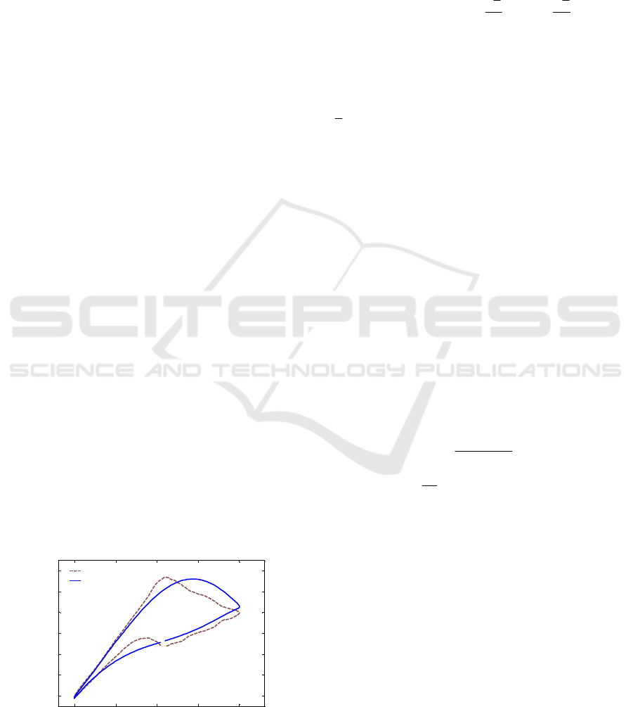
Figure 1: Linear aerodynamic model.
wind-tunnel data of the longitudinal forced pitch
oscillations in Fig. 1.
Linear model is a conventional aerodynamic
model. In many practical cases, the aerodynamic
forces and moments are approximated by linear
terms in their Taylor series expansions. In the case
of lift coefficient, the function is defined as follows:
() () ()
22
LLs Lq L
qc c
CC C C
VV
α
α
αα α
=+ +
(1)
Where
L
C
is the total lift coefficient,
L
s
C
denotes the static lift coefficient.
, q
α
are angle of
attack and pitch angle rate separately.
,
L
qL
CC
α
are
corresponding dynamic factors.
V
presents air speed,
c
is the wing mean geometric chord. Linear model
assumes that aerodynamic forces and moments
depend only on the instantaneous values of the flight
states. Due to lacking the considerations of unsteady
aerodynamic effects, the outputs of linear model
often contain notable error at high angles of attack
comparing to the wind-tunnel data (Fig. 1).
2.2 State-space Model
The state-space model takes time delay of flow
separation and reattachment into account. An
internal variable which describes the flow state is
introduced by (Goman et al., 1994) to express time
delay of unsteady aerodynamics at high angles of
attack. This internal state variable is called the
longitudinal position of the separation point
x
. The
movement of the separation point for unsteady flow
conditions is defined as follows:
0
(*)
102
1
()
1
()
x
e
dx
xx
dt
σα α
α
τατα
−
=
+
+= −
(2)
Function
0
()x
α
is the static variation which
depends on the instantaneous angle of attack
α
.
*
α
is defined as the angle of attack when separation
point reaches the middle of airfoil chord,
σ
is slope
factor.
The unsteady fluid mechanics processes are
divided into two groups. The first group is the quasi-
steady effects such as circulation and boundary-layer
convection lags, which tend to delay flow separation
or burst onset by an amount roughly proportional to
the pitch rate. This combined effect is expressed as
an argument shift
02
()x
ατα
−
. Where the parameter
2
τ
defines the total time delay associated with the
above effects. The second group of flow phenomena
0 20 40 60 80
0
0.5
1
1.5
2
2.5
3
Lift coefficient
Angle of attack/deg
Linear Model
Wind-Tunnel Data
Aircraft Unsteady Aerodynamic Hybrid Modeling Based on State-Space Representation and Neural Network
233

define the transient aerodynamic effects, in which
any disturbance of the separated flow is followed by
an adjustment or relaxation back to the steady-state.
The adjustment process is governed by a first-order
ordinary differential equation (Formula 2) with
relaxation time constant
1
τ
.
The solid line and dashed lines show the
variations of the separation point position for steady
and unsteady conditions separately in Fig. 2. The
difference between solid line and dashed lines
causes the pneumatic hysteresis of unsteady
aerodynamics.
Figure 2: Instantaneous separation point variations.
In state-space model, aerodynamic forces and
moments depend on not only the instantaneous
values of the flight states, but also the instantaneous
separation point position that can differ considerably
from its stationary value. Since the pitch oscillations
are considered with
q
α
=
, the effects of
α
are no
longer included in the subsequent longitudinal
unsteady aerodynamic coefficient expressions. The
corresponding unsteady lift coefficient state-space
representation is:
() (,,)
LLs Ld
CC C qx
αα
=+
(3)
The static coefficient
L
s
C
is conventionally
approximated with the first three items in its Taylor
series expansion, while the dynamic coefficient
L
d
C
is approximated with the first five items in its Taylor
series expansion.
2
2
2
2
00 0
2
2
() ()
() () ()
2
() ()
22
Ls Ls Ls
Ls
Ld L Lq
L
Lq
Lq
CC Cx Cx
qc
CCxCx Cx
V
qc qc
Cx C x
VV
α
α
α
α
α
αα
αα
α
=+ +
=+ + +
+
(4)
All the corresponding factors in both the static
coefficient and the dynamic coefficient can be
expressed with second-order polynomial functions,
like
L
s
C
α
and
L
C
α
in the lower formula.
2
001020
2
01 2
()
()
Lsa Ls Ls Ls
LLLL
Cx k kxkx
Cx k kxkx
αα α
αααα
=+ +
=+ +
(5)
Where
012
,,
Ls Ls Ls
kkk
ααα
and
012
,,
LLL
kkk
ααα
are
unknown parameters in the polynomial aerodynamic
model. Totally, 26 parameters should be determined
for the lift coefficient state-space representation,
including four parameters
*
12
,,,
σα τ τ
in the
separation point model (Formula 2) and all the
relevant factors in the polynomial model (Formula
5).
2.3 State-space Model Evaluation
Suitable simulations of the maneuvers in the wind
tunnels are important for understanding the physics
of complex flow phenomena (Hosder et al., 2007).
These maneuvers should allow the physical
simulation of aircraft dynamic behavior, which is
subject to the dynamic similarity of the aircraft
model, and identification of the aircraft aerodynamic
model structure and its parameters (Pattinson et al.,
2013). For the case of symmetrical motion of the
wing in the longitudinal plane, pitch-only oscillation
has been successfully used to characterize unsteady
aerodynamics at high angles of attack (Pattinson et
al., 2012). In this paper, Forced large-amplitude
pitch oscillations are executed in the wind tunnel.
The corresponding experimental data of
aerodynamic forces and moments are collected and
used to estimate the aerodynamic models.
Harmonic motions in pitch oscillations with a
fixed center of gravity are implemented:
0
sin(2 )
2cos(2)
Aft
qfA ft
αα π
αππ
=−
==−
(6)
Oscillations were carried out with amplitude
40A
ο
=
and different pitching frequencies
f
. The
initial angle of attack
0
α
is set to
40
ο
, so the angle
of attack
α
varies from
0
ο
to
80
ο
. Lift coefficient
and pitch moment coefficient data at
0.4
f
Hz=
,
0.6
f
Hz=
and
0.8
f
Hz=
are used to testify the
validity of the state-space model. After a proper
parameter optimization for lift and pitch moment
state-space models with Nelder-Mead method and
particle swarm optimization method, the
comparisons between optimized state-space model
and corresponding wind-tunnel data are partly
shown in the following figures:
0 10 20 30 40 50 60 70 80
0
0.2
0.4
0.6
0.8
1
Angle of attack/deg
Instantaneous separation point x
x
0
(
α
)
ICPRAM 2016 - International Conference on Pattern Recognition Applications and Methods
234
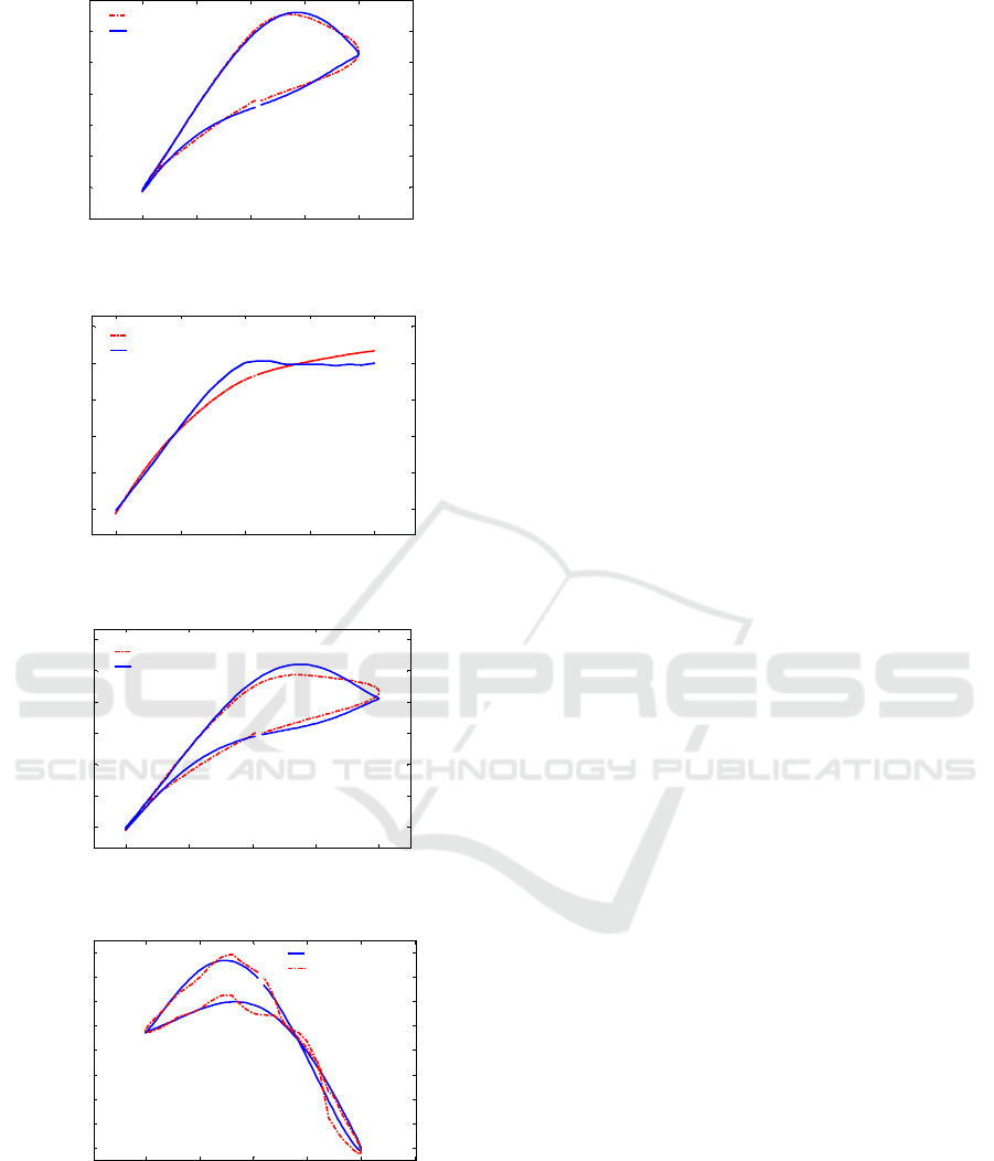
Figure 3: Lift coefficient response at f=0.6Hz.
Figure 4: Static lift coefficient response.
Figure 5: Lift coefficient response at f=0.4Hz.
Figure 6: Pitch moment coefficient response at f=0.6Hz.
The figures above reveal that state-space model
can approximate the wind-tunnel experimental data
to a certain extent. Fig. 5 and Fig. 6 show that
though state-space model can effectively reflect time
delay characteristics of unsteady aerodynamics at
high angles of attack, the model responses are not
always in good agreement with the wind-tunnel data.
The polynomial model is not accurate enough to
describe the nonlinear static aerodynamic coefficient,
like the static lift coefficient in Fig. 4.
Goman’s nonlinear differential equation concept
provides the most promising combination of relative
simplicity, retention of physical significance in its
parameters, and ability to model a wide range of
common flow features (Greenwel et al., 2004).
However, modifications should be added to state-
space model to capture more accurate and reliable
unsteady aerodynamic responses.
3 HYBRID MODEL
Neural networks (NN) have recently been shown to
be an effective tool for modeling nonlinear unsteady
aerodynamics regardless of the aircraft
configurations. In previous studies, a simple time
delay is generally added to the flight states
instantaneous values as the input signals in unsteady
aerodynamic NN model. Though sometimes these
NN models can achieve good accuracy due to the
excellent approximating performance, actual
physical mechanism of unsteady aerodynamics is
not clearly reflected and the NN models are usually
oversized with redundant neurons. As a meaningful
attempt in this paper, a hybrid model which
combines state-space representation and back-
propagation neural network is presented to integrate
respective advantages in these two models.
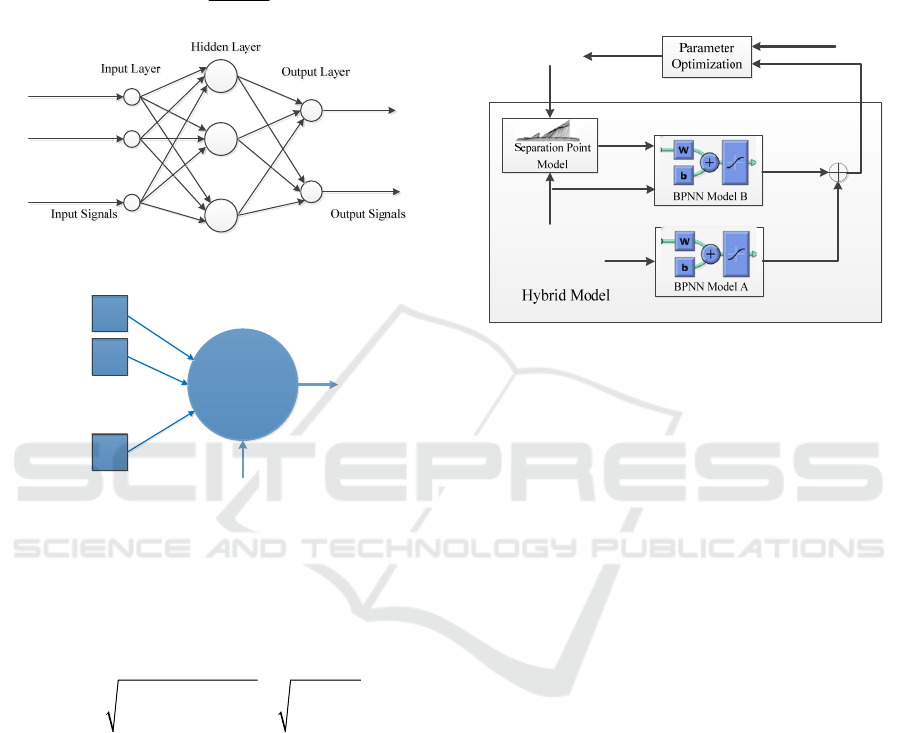
3.1 Back-propagation Neural Network
Back-propagation neural networks (BPNN) are the
most widely applied neural network models. The
structure of generalized three-layer neural network
consists of the input layer, the hidden layer and the
output layer (Fig. 7). The node in the neural network
is called the neuron. Each neuron receives signals
from the neurons in the previous layer, and
calculates its output through a specific transfer
function.
Fig. 8 shows the typical neuron transfer model.
For nodes in the hidden layer, input signals are
(1,2,...,)
j
x
jn=
. These signals are summed with
weight values
j
w
corresponding to the signal
connections. Bias value
s
is added to the weighted
sum of the input signals to generate a summed value
net
. The final output
g
of the node is mapped
through a commonly used hyperbolic tangent
-20 0 20 40 60 80 100
-0.5
0
0.5
1
1.5
2
2.5
3
Angle of attack/deg
Lift coefficient
State-Space Model
Wind-Tunnel Data
0 20 40 60 80
0
0.5
1
1.5
2
2.5
Angle of attack/deg
Static lift coefficient
State-Space Model
Wind-Tunnel Data
0 20 40 60 80
0
0.5
1
1.5
2
2.5
3
Angle of Attack/deg
Lift coefficient
State-Space Model
Wind-Tunnel Data
0 20 40 60 80 100
-0.25
-0.2
-0.15
-0.1
-0.05
0
0.05
0.1
0.15
Angle of attack/deg
Pitch moment coefficient
Wind-Tunnel Data
State-Space Model
Aircraft Unsteady Aerodynamic Hybrid Modeling Based on State-Space Representation and Neural Network
235
sigmoid transfer function as the nonlinear activation
function. The nodes in the output layer share the
same scheme as the nodes in the hidden layer.
1
2et
2
() 1
1
n
jj
j
n
net x w s
gfnet
e
=
−
=+
== −
+
∑
(7)
1
x
i
i
i
i
1
g
1
y
h
y
i
i
i
i
i
i
2
x
l
x
2
g
n
g
Figure 7: Generalized neural network structure.
1
.
n
jj
j
x
ws
=
+
∑
s
g
1
x
2
x
n
x
2
w
n
w
1
w
Figure 8: Typical neuron transfer model.
To minimize the mean-squared error
E
between
BPNN model response
B
j
y
and the actual response
R
j
y
, the error value
j
e
is propagated backwards
through the network for weight values and bias
values updates.
22
11
min ( ) / /
NN
Bj Rj j
jj
EyyNeN
==
=− =
∑∑
(8)
Gradient descent method is used in the back-
propagation neural network for parameter learning.
When the mean-squared error decreases and reaches
a given threshold range, parameter optimization
stops and the BPNN model is regarded as an
acceptable approximator to the actual model.
3.2 Hybrid Model Structure
To obtain a more accurate and reliable unsteady
aerodynamic model and reflect actual flow
separation characteristics, the unsteady aerodynamic
hybrid model is proposed in this paper. As the
differential equation of the separation point can be
used to simulate time delay of unsteady aerodynamic
responses, the separation point model is reserved in
the hybrid model. As far as model accuracy and
output response approximation are concerned, back-
propagation neural network is introduced to replace
the conventional polynomial model. The structure of
unsteady aerodynamic hybrid model is shown in the
following figure.
()t
α
()
Ls
Ct
()
x
t
*
12
,,,
σα τ τ
()
Ld
Ct
*
()
L
Ct
() ()tt
αα
()
L
Ct
Figure 9: Unsteady aerodynamic hybrid model structure.
Fig. 9 shows that in lift coefficient unsteady
hybrid model, the static lift coefficient and the
dynamic lift coefficient are identified separately. As
the static coefficient only depends on the angle of
attack, a simple BPNN model A is adopted to
describe the nonlinear steady mapping between
these two variables. For the dynamic lift coefficient,
the separation point model is firstly used to generate
the separation point
x
from
α
and
α
. Subsequently,
BPNN model B is introduced with
,
αα
and
x
as
input signals to simulate the unsteady lift component.
The dynamic lift coefficient
L
d
C
is added to the
static lift coefficient
L
s
C
to form the total lift
coefficient response
L
C
. Finally,
L
C
is compared to
the wind-tunnel lift coefficient data to optimize the
relevant parameters in the hybrid model.
3.3 Hybrid Model Optimization
Two sets of unknown parameters exist in the
unsteady aerodynamic hybrid model. Four
parameters
*
12
,,,
σα τ τ
in the separation point model
decide the separation point dynamic characteristics,
while all the relevant weight values and bias values
in BPNN model reveal the nonlinear mapping
function of the unsteady aerodynamic forces and
moments. All of the above unknown parameters
should be identified and optimized to realize the best
model response.
ICPRAM 2016 - International Conference on Pattern Recognition Applications and Methods
236
For the unknown values in BPNN model A, a
direct gradient descent method is taken to optimize
the corresponding parameters. When it comes to the
dynamic aerodynamic component identification, a
nested parameter optimization algorithm is used.
The four parameters
*
12
,,,
σα τ τ
are optimized as the
outside loop of the nested optimization structure, the
corresponding optimization algorithms are Nelder-
Mead method and particle swarm optimization
method. The relevant weight values and bias values
in BPNN model B are identified with gradient
descent method as the inner loop. The nested
parameter optimization structure is as follows:
()
Ls
Ct
()
x
t
*
12
,,,
σα τ τ
()
Ld
Ct
*
()
L
Ct
() ()tt
αα
()
L
Ct
J
Figure 10: Nested parameter optimization structure.
In the case of dynamic lift coefficient
identification, the optimal objective function is
defined as the mean-squared error between the
hybrid model response and the wind-tunnel data, as
shown in the following formula.
*2
1
min ( ) /
N
Lj Lj
j
J
CC N
=
=−
∑
(9)
As far as the number of the hidden layer neurons
is concerned, an oversized network could overfit and
overlearn for a special data set. Conversely, an
undersized network with too few hidden layer
neurons could significantly reduce the results
accuracy (Boëly et al., 2010). For the parameter
identification of the hybrid model, a large enough
integer value is chosen as the number of the hidden
layer neurons to ensure the model response accuracy.
After the parameters
*
12
,,,
σα τ τ
are determined with
the oversized BPNN model B, a model
simplification process is executed to reduce the
redundant neurons. Useless and redundant neurons
are deleted one-by-one and the parameters in BPNN
model B are readjusted until the mean-squared error
J
exceeds the pre-determined threshold. Finally, a
simplified hybrid model is achieved without
lowering model accuracy criterion.
4 SIMULATION RESULTS
The considered unsteady aerodynamic hybrid model
is tested using the wind-tunnel experimental data. As
it is mentioned in Section 2, the lift coefficient and
pitch moment coefficient data come from the forced
large-amplitude pitch oscillations at
0.4
f
Hz=
,
0.6
f
Hz=
and
0.8
f
Hz=
. Two thirds of the
experimental data are used to train the neural
networks in the hybrid model, and one third of the
experimental data are used to evaluate the hybrid
model performance.
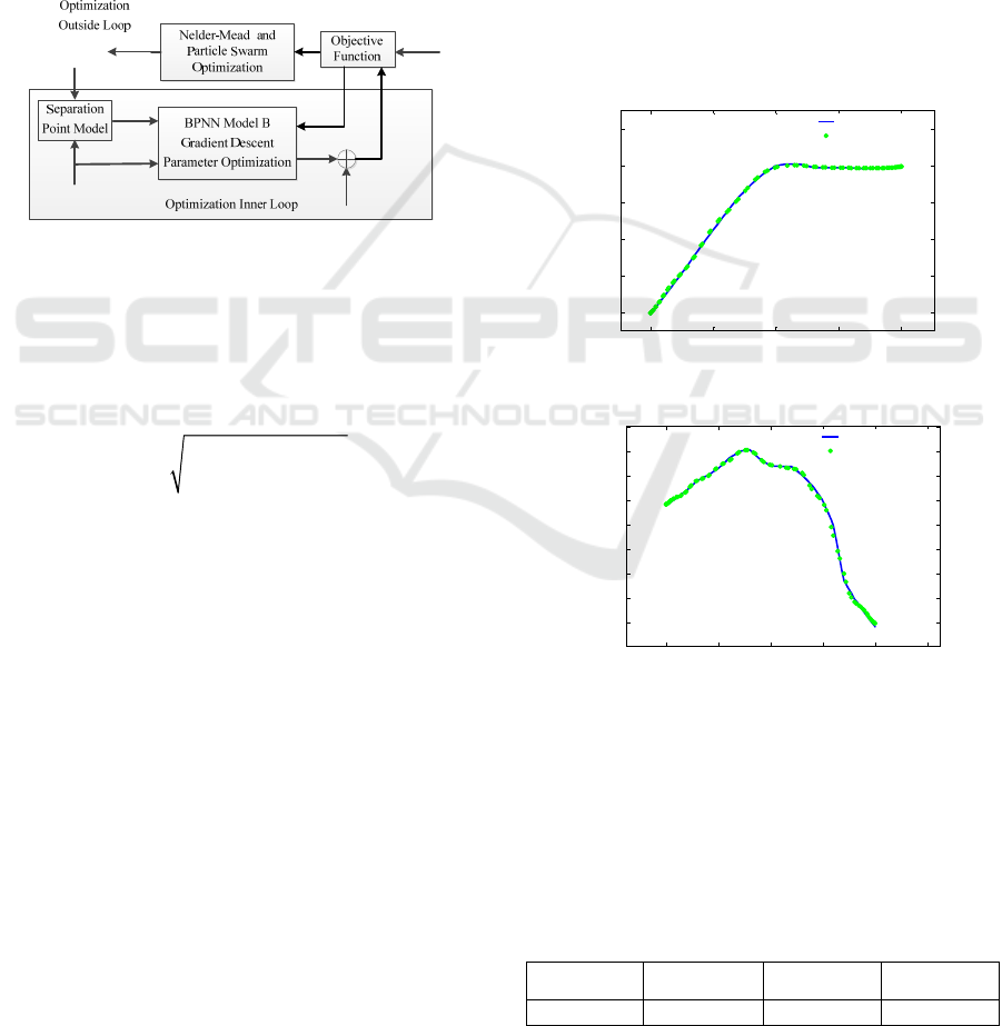
For the hidden layer in BPNN model A, 6
neurons are enough to create a more accurate static
aerodynamic model comparing to state-space model.
The responses of the static BPNN models are
illustrated in Fig. 11 and Fig. 12.
Figure 11: Static lift coefficient response.
Figure 12: Static pitch moment coefficient response.
As for the identifications of the dynamic
aerodynamic component, 30 hidden layer neurons
are set as the initial size of BPNN model B. The
four parameters
*
12
,,,
σα τ τ
are firstly identified
using the nested optimization algorithm mentioned
in Section 3.
Table 1: Identification results in separation point model.
σ
*
/deg
α
1
/
s
τ
2
/
s
τ
0.11 41.2 0.042 0.047
0 20 40 60 80
0
0.5
1
1.5
2
2.5
Angle of attack/deg
Static lift coefficient
Wind-Tunnel Data
BPNN Model
0 20 40 60 80 100
-0.25
-0.2
-0.15
-0.1
-0.05
0
0.05
0.1
0.15
Angle of attack/deg
Static pitch moment coefficient
Wind-Tunnel Data
BPNN Model
Aircraft Unsteady Aerodynamic Hybrid Modeling Based on State-Space Representation and Neural Network
237
Subsequently, model simplification process is
carried out to reduce the redundant neurons. The
simplification results indicate that 6 hidden layer
neurons are accurate enough to represent the
nonlinear mapping relation in BPNN model B for
lift coefficient modeling. As for the pitch moment
coefficient, 7 hidden layer neurons are necessary to
guarantee model accuracy. The optimized unsteady
aerodynamic hybrid models are compared with the
conventional state-space models. The mean-squared
errors
J
are listed in Table 2. SS-M is short for
state-space model, CH-M denotes the complicated
hybrid model with 30 hidden layer neurons, SH-M
represents the simplified hybrid model.
Table 2: Mean-squared error comparisons.
2
/10J
−
f=4Hz f=6Hz f=8Hz
Lift
coefficient
SS-M 7.87 4.58 8.66
CH-M 3.05 1.34 2.47
SH-M 3.32 1.61 3.46
Pitch
moment
coefficient
SS-M 4.79 4.12 11.1
CH-M 0.42 0.35 0.40
SH-M 1.05 0.56 0.57
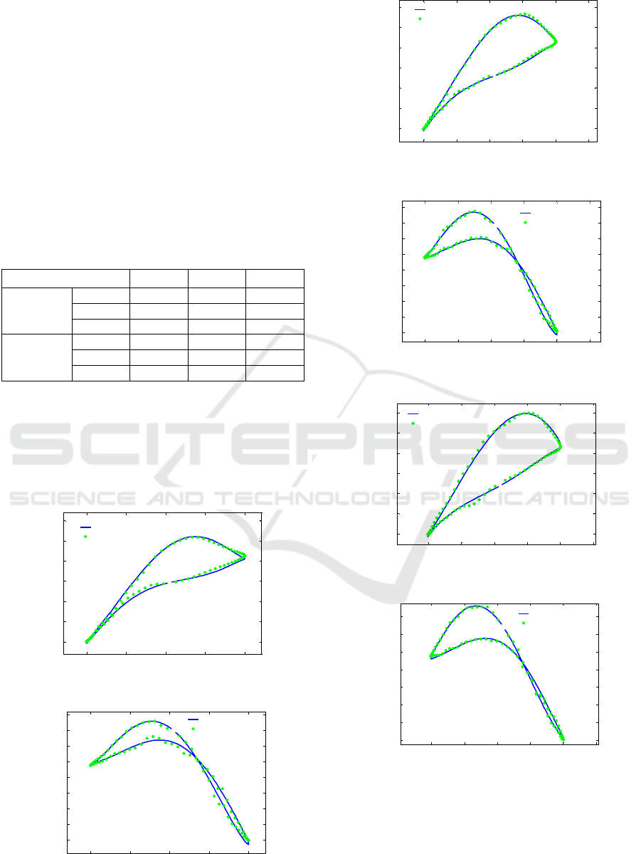
Comparing to conventional state-space model,
the hybrid model can achieve obvious accuracy
improvement in approximating the unsteady
aerodynamic response. The response results of the
simplified hybrid models achieve good agreements
with different wind-tunnel experimental data, which
are illustrated in the following figures.
Figure 13: Lift coefficient response at f=0.4Hz.
Figure 14: Pitch moment coefficient response at f=0.4Hz.
Figure 15: Lift coefficient response at f=0.6Hz.
Figure 16: Pitch moment coefficient response at f=0.6Hz.
Figure 17: Lift coefficient response at f=0.8Hz.
Figure 18: Pitch moment coefficient response at f=0.8Hz.
5 CONCLUSIONS
A hybrid model which combines state-space
representation and back-propagation neural network
0 20 40 60 80
0
0.5
1
1.5
2
2.5
3
Angle of attack/deg
Lift coefficient
Wind-Tunnel Data
Hybrid Model
0 20 40 60 80
-0.25
-0.2
-0.15
-0.1
-0.05
0
0.05
0.1
0.15
Angle of attack/deg
Pitch moment coefficient
Wind-Tunnel Data
Hybrid Model
0 20 40 60 80 100
0
0.5
1
1.5
2
2.5
3
Angle of attack/deg
Lift coefficient
Wind-Tunnel Data
Hybrid Model
0 20 40 60 80 100
-0.25
-0.2
-0.15
-0.1
-0.05
0
0.05
0.1
0.15
Angle of attack
Pitch moment coefficient
Wind-Tunnel Data
Hybrid Model
0 20 40 60 80 100
0
0.5
1
1.5
2
2.5
3
Angle of attack/deg
Lift coefficient
Wind-Tunnel Data
Hybrid Model
0 20 40 60 80 100
-0.25
-0.2
-0.15
-0.1
-0.05
0
0.05
0.1
Angle of attack/deg
Pitch moment coefficient
Wind-Tunnel Model
Hybrid Model
ICPRAM 2016 - International Conference on Pattern Recognition Applications and Methods
238

is proposed in this paper to describe the aircraft
unsteady aerodynamic characteristics. According to
the simulation results, the conventional state-space
model has limited approximation quality in
modeling unsteady aerodynamics. For the purpose of
improving model accuracy and universality, back-
propagation neural network is introduced and
replaces the polynomial model in state-space
representation. The unsteady aerodynamic hybrid
model is identified and optimized with nested
optimization algorithm using the wind-tunnel data in
forced large-amplitude pitch oscillation experiments.
With satisfactory similarity to the wind-tunnel data,
the hybrid model presented in this paper is validated
to be effective in both reflecting unsteady time delay
characteristics and representing complex nonlinear
mapping relation for unsteady aerodynamics at high
angles of attack.
ACKNOWLEDGEMENTS
This work was made possible thanks to the support
of Science and Technology on Aircraft Control
Laboratory.
REFERENCES
Boëly, N., Botez, R. M., 2010. New approach for the
identification and validation of a nonlinear F/A-18
model by use of neural networks. IEEE Transactions
on Neural Networks, 21(11):1759–1765.
Chen, G., Xu, M., and Chen, S. L., 2004. Reduced-order
model based on volterra series in nonlinear unsteady
aerodynamics. Journal of Astronautics, 25(5): 492–
295.
Goman, M., Khrabrov, A., 1994. State-space
representation of aerodynamic characteristics of an
aircraft at high angles of attack. Journal of
Aircraft, 31(5):1109-1115.
Greenwell, D. I., 2004. A Review of Unsteady
Aerodynamic Modeling for Flight Dynamics of
Manoeuvrable Aircraft. In AIAA Atmospheric Flight
Mechanics Conference and Exhibit, Paper 2004-5276.
Hosder, S., Simpson, R. L., 2007. Experimental
investigation of unsteady flow separation on a
maneuvering axisymmetric body. Journal of aircraft,
44(4): 1286–1295.
Ignatyev, D. I., Khrabrov, A. N., 2015. Neural network
modeling of unsteady aerodynamic characteristics at
high angles of attack. Aerospace Science and
Technology, 41: 106–115.
Kumar, R., Ghosh, A. K., 2011. Nonlinear Longitudinal
Aerodynamic Modeling Using Neural Gauss-Newton
Method. Journal of Aircraft, 48(5): 1809–1813.
Kumar, R., Mishra, A., Ghosh, A. K., 2012. Nonlinear
Modeling of Cascade Fin Aerodynamics Using
Kirchhoff's Steady-State Stall Model. Journal of
Aircraft, 49(1): 315–319.
Pattinson, J., Lowenberg, M. H., Goman, M. G., 2012.
Multi-Degree-of-Freedom Wind-Tunnel Maneuver
Rig for Dynamic Simulation and Aerodynamic Model
Identification. Journal of Aircraft, 50(2): 551–566.
Pattinson, J., Lowenberg, M. H., Goman, M. G. 2013.
Investigation of Poststall Pitch Oscillations of an
Aircraft Wind-Tunnel Model. Journal of
Aircraft, 50(6): 1843–1855.
Sun, W., Gao, Z., Du, Y., Xu, F., 2015. Mechanism of
unconventional aerodynamic characteristics of an
elliptic airfoil. Chinese Journal of Aeronautics, 28(3):
687–694.
Wang, B. B., Zhang, W. W., Ye, Z. Y., 2010. Unsteady
Nonlinear Aerodynamics Identification Based on
Neural Network Model. Acta Aeronautica Et Sinica,
31(7): 1379–1388.
Wang, Q., Qian, W., He, K., 2015. Unsteady aerodynamic
modeling at high angles of attack using support vector
machines. Chinese Journal of Aeronautics, 28(3):
659–668.
Williams, D. R., Reißner, F., Greenblatt, D., Müller-Vahl,
H., Strangfeld, C., 2015. Modeling Lift Hysteresis
with a Modified Goman-Khrabrov Model on Pitching
Airfoils. In 45th AIAA Fluid Dynamics Conference,
Paper 2015-2631.
Zakaria, M. Y., Taha, H. E., Hajj, M. R., Hussein, A. A.,
2015. Experimental-Based Unified Unsteady
Nonlinear Aerodynamic Modeling For Two-
Dimensional Airfoils. In 33rd AIAA Applied
Aerodynamics Conference
, Paper 2015-3167.
Aircraft Unsteady Aerodynamic Hybrid Modeling Based on State-Space Representation and Neural Network
239
