GPS Trajectory Data Enrichment based on a Latent Statistical Model

Akira Kinoshita

, Atsuhiro Takasu

, Kenro Aihara

, Jun Ishii

, Hisashi Kurasawa

, Hiroshi Sato

Motonori Nakamura

and Jun Adachi

The University of Tokyo, 2-1-2 Hitotsubashi, Chiyoda, Tokyo, Japan

National Institute of Informatics, 2-1-2 Hitotsubashi, Chiyoda, Tokyo, Japan

NTT Network Innovation Laboratories, 3-9-11 Midoricho, Musashino, Tokyo, Japan

Keywords:

GPS Trajectory Data, Interpolation, Latent Statistical Model, Moving Mode Estimation.

Abstract:

This paper proposes a latent statistical model for analyzing global positioning system (GPS) trajectory data.

Because of the rapid spread of GPS-equipped devices, numerous GPS trajectories have become available,

and they are useful for various location-aware systems. To better utilize GPS data, a number of sensor data

mining techniques have been developed. This paper discusses the application of a latent statistical model

to two closely related problems, namely, moving mode estimation and interpolation of the GPS observation.

The proposed model estimates a latent mode of moving objects and represents moving patterns according to

the mode by exploiting a large GPS trajectory dataset. We evaluate the effectiveness of the model through

experiments using the GeoLife GPS Trajectories dataset and show that more than three-quarters of covered

locations were correctly reproduced by interpolation at a ﬁne granularity.

1 INTRODUCTION

Because of the rapid spread of mobile devices

equipped with a global positioning system (GPS),

location information is combined with a wide vari-

ety of data and effectively exploited to realize new

location-aware systems as well as to make existing

systems smarter. For example, recommender systems

utilize GPS data in several tasks, such as location-

aware shopping recommendations (Yang et al., 2008)

and tourism recommendations (Cao et al., 2010).

Location information is key information for intelli-

gent transportation systems such as trafﬁc monitoring

(Schnitzler et al., 2014) and incident detection (Ki-

noshita et al., 2015).

To utilize location information effectively, a num-

ber of sensor data mining methods have been pro-

posed, with the moving mode estimation method of-

ten discussed in the literature. When analyzing user

behavior, the means of traveling are useful. How-

ever, most GPS data do not contain such informa-

tion. Zheng et al. (Zheng et al., 2010a) proposed a

mode-prediction method in which they ﬁrst detected

a mode-change point in a trajectory and then assigned

a mode to each segment of the trajectory. Latent vari-

ables are often introduced to detect the mode. Yu

et al. (Yu and Kobayashi, 2003) proposed a moving

mode prediction method based on an extended hid-

den Markov model (HMM) where a moving mode is

represented by a hidden state of the HMM. They as-

sumed that the modes represent purposes and means

of traveling such as driving, shopping, etc.

There has also been a growing interest in trajec-

tory pattern mining. Giannotti et al. (Giannotti et al.,

2007) proposed a frequency-based method, where

they found popular areas and frequent moving pat-

terns from trajectories. Monreale et al. (Monreale

et al., 2009) extended this study for location predic-

tion. They extracted the moving pattern represented

by tree-structured data called a T-pattern tree from the

training data, and then predicted the position based on

the moving patterns.

Although the amount of GPS data is extremely

large, we still need to enrich the data in various as-

pects. For example, the sampling rate is limited for

saving the consumption of energy, which causes a

sparsity problem for some analyses. Sampling every

few seconds, for instance, is not sufﬁcient for identi-

fying the route of a car that is moving fast. In addi-

tion, some sensing data could be missing because of

transmission failure.

This paper discusses two GPS data enrichment

Kinoshita, A., Takasu, A., Aihara, K., Ishii, J., Kurasawa, H., Sato, H., Nakamura, M. and Adachi, J.

GPS Trajectory Data Enrichment based on a Latent Statistical Model.

DOI: 10.5220/0005699902550262

In Proceedings of the 5th International Conference on Pattern Recognition Applications and Methods (ICPRAM 2016), pages 255-262

ISBN: 978-989-758-173-1

255

problems, namely, interpolation of GPS trajectories

and traveling mode estimation.

When the sampling frequency is not high enough

for analysis, GPS trajectories are interpolated in space

and time. From the spatial point of view, there are

several approaches to estimate locations and paths of

GPS data. Many of them form a trajectory curve

from discrete GPS position data. Brunsdon (Bruns-

don, 2007) applied a principal curve detection tech-

nique (Biau and Fischer, 2012) to trace paths from

GPS data. Sankararaman et al. (Sankararaman et al.,

2013) extracted trajectory curve segments from tra-

jectories, where a frequent portion of the trajectories

is extracted by the dynamic time warping-based sim-

ilarity. When moving objects are supposed to be on

the road, map matching is useful for interpolation,

and many studies have investigated the map-matching

problem. Feng and Timmermans (Feng and Tim-

mermans, 2013) proposed a map-matching method

of GPS data based on the Bayesian belief network.

Karagiorgou and Pfoser (Karagiorgou and Pfoser,

2012) proposed a map generation method where they

detected intersections and then made a road network

by connecting them. Hao et al. (Hao et al., 2014)

proposed a probabilistic model to estimate the vehi-

cle driving state, such as idling and acceleration, to

estimate precisely the location at any time.

From the temporal point of view, Yang et al. (Yang

et al., 2013) proposed the extended Gaussian mixture

model (GMM) to estimate the traveling time of vehi-

cles, where GMM is used to represent the probability

density function of traveling time. Wang et al. (Wang

et al., 2014) proposed a tensor-based method of trav-

eling time.

The present paper proposes a statistical model for

interpolating GPS sensing points. It introduces trav-

eling modes to describe a movement behavior that

varies according to the transportation means, with the

expectation of improvement in interpolation accuracy.

To exploit the training trajectories labeled with trav-

eling modes, we applied the semi-supervised learning

technique to obtain an effective model and evaluated

the model effectiveness using real data.

2 MODEL FOR GPS

TRAJECTORY ENRICHMENT

2.1 Trajectory

As moving objects generally travel on a road, ob-

served GPS points are often mapped onto the road

by a map-matching technique (e.g., (Goh et al., 2012;

Wei et al., 2012)). However, the observed location is

usually erroneous and the map-matching result is not

always correct. In addition, people sometimes get out

of the road network such as in a park. Therefore, we

describe the location of moving objects by a grid. We

ﬁrst partition a 2-dimensional space into cells each

of which represents an equal-sized and mutually ex-

cluded rectangle. Let G denote the grid, i.e., the set of

cells in which objects move. We represent the loca-

tion of a moving object by a cell g ∈ G, meaning that

the object is somewhere in the cell.

Given a grid G, the movement of a moving object

is described by the cells it passes through and by the

traveling time for each cell. Let g

be the i-th cell that

the object passes through. Once the object enters a

cell g

, it travels in it for time t

, then moves to the next

cell g

i+1

. Therefore, the trajectory of a moving object

is deﬁned as a pair (g, t), where g

= hg

, g

, . . . , g

i is

a location sequence, t

= ht

, t

, . . . , t

i is a traveling

time sequence, and l is the length of both sequences.

2.2 Traveling Mode

Moving objects, particularly people, change location

by walking or by various means of transportation such

as a vehicle. Even when an object moves by the same

means, its behavior may be different according to its

location. For example, people tend to walk quickly in

a business district to go to work, whereas they tend

to walk more slowly in a commercial district. We in-

troduce a set M of modes to distinguish the behavior

patterns. Note that the mode is latent because we can-

not observe it explicitly. A moving object may change

its traveling mode at any time while traveling, but it

makes the model too complicated. Therefore, in this

paper, we assume that the moving object travels with

the same mode in a cell. The traveling mode depends

on the location. For example, the “train” mode is

likely to be chosen on a railway, while the “car” mode

is likely to be chosen on an expressway. Therefore,

for each cell g, we introduce a multinomial probabil-

ity distribution with parameter θ

= (θ

)

m∈M

. The

probability of the traveling mode m ∈ M of an object

in a cell g is:

p(m | g)

= θ

. (1)

2.3 Traveling Time of Moving Objects

The traveling time varies according to the traveling

mode and location as well as the individual charac-

teristics. To avoid the sparsity problem in parameter

estimation, we ignore the differences between indi-

viduals. For each mode m in a cell g, we describe the

distribution of traveling time t in terms of a univari-

ICPRAM 2016 - International Conference on Pattern Recognition Applications and Methods

256

ate Gaussian distribution with mean µ

and variance

, i.e.,

p(t | g, m)

= N (t; µ

, σ

)

2πσ

exp



−

(t − µ

)

2σ



. (2)

Taking a marginal distribution, the traveling time t to

pass through g follows a Gaussian mixture distribu-

tion:

p(t | g) =

∑

m∈M

N (t;µ

, σ

). (3)

2.4 Moving Direction

To predict the future location of a moving object, we

introduce a probability distribution for the next cell to

move into.

Suppose a moving object is in a cell g and consider

the probability distribution over the adjacent cells.

The probability distribution should depend on the cell

itself because of trafﬁc constraints such as “no right

turn” and attractors such as popular shops. It should

also depend on the traveling mode. If a moving ob-

ject is traveling by train, it tends to go straight to the

next cell. On the other hand, if the moving object is

walking, it may move to various directions.

From this observation, we introduce the probabil-

ity distribution of the direction of an adjacent cell to

which a moving object moves. Let D be a set of di-

rections of adjacent cells: {north, east, south, west}.

When a moving object in mode m is in a cell g, we as-

sume that its moving direction d ∈ D follows a multi-

nomial distribution with parameter φ

= (φ

gmd

)

d∈D

namely,

p(d | g, m)

= φ

gmd

. (4)

Now, the trajectory of a moving object is redeﬁned as

a triple (g, t, d), where d

= hd

, d

, . . . , d

i is the mov-

ing direction sequence and d

is the moving direction

from the i-th cell g

2.5 Likelihood of a Trajectory

Let x

= (g, t, d) be a trajectory. The moving object

takes only one of the traveling modes for each cell,

although they are latent. Let m

be the traveling mode

in the i-th cell and y

= hm

, m

, . . . , m

i be the mode

sequence for the trajectory x. Then, the complete-data

likelihood of the model is given as follows:

p(x, y) =

∏

i=1

p(t

| g

, m

) · p(d

| g

, m

) · p(m

| g

)

∏

i=1

N (t

;µ

, σ

) · θ

· φ

. (5)

3 PARAMETER ESTIMATION

We adopt a maximum a posteriori (MAP) estimation

for learning the prediction model. Let us ﬁrst intro-

duce the conjugate priors for each probability distri-

bution. The symmetric Dirichlet distribution with the

parameter α (respectively β) is used for the multino-

mial distributions for the mode (respectively the mov-

ing direction), whereas the Gaussian-gamma distribu-

tion with the parameters ν, η, a, and b is used for

the traveling time distribution. Now the generative

process of the model parameters is to choose them as

follows:

1. θ

∼ Dir(α) for each g ∈ G,

2. φ

∼ Dir(β) for each g ∈ G and m ∈ M,

3. (µ

, (σ

)

−1

) ∼ GaussianGamma(ν, η, a, b) for

each g ∈ G and m ∈ M.

The observed trajectory data are considered to be

generated under these parameters. Most of them are

unlabeled, i.e., their mode is unknown. Let X

denote

a set of unlabeled trajectories. The generative process

of X

is as follows.

4. For each observation in each trajectory in X

(a) m ∼ Multi(θ

(b) d ∼ Multi(φ

, σ

On the other hand, we can obtain a portion of labeled

data where the mode of observation is known as in the

GeoLife dataset (Zheng et al., 2009). Let X

denote a

set of labeled trajectories. The generative process of

is as follows.

5. For each observation in each trajectory in X

(a) d ∼ Multi(φ

(b) t ∼ N (µ

, σ

where m is the labeled mode.

For simplicity, we denote the set of parameters

used in our model by Θ:



{θ

}

g∈G

, {φ

, µ

, σ

}

g∈G,m∈M



. (6)

Using both labeled and unlabeled data, Θ can be esti-

mated by solving the following formula including two

weight parameters λ

and λ

that control the effect

of labeled and unlabeled data, respectively (Gr

onroos

et al., 2014):

arg max

[ln p(Θ) + λ

ln p(X

| Θ) + λ

ln p(X

| Θ)].

(7)

Although we are in a semi-supervised situation, the

estimate of Θ can be computed by an expectation–

maximization (EM) algorithm. In the remainder of

GPS Trajectory Data Enrichment based on a Latent Statistical Model

257

this section, we derive the MAP estimator, concentrat-

ing on differences from the ordinary textbook treat-

ments (Bishop, 2006; Zhu and Goldberg, 2009) be-

cause of lack of space.

The Q function for our model is given by

Q(Θ,

Θ) =

∑

x∈X

|x|

∑

i=1

∑

m∈M

p(m | x

Θ)ln p(x

, m | Θ),

(8)

where

p(m | x

Θ) ∝

· N (t

| ˆµ

), (9)

p(x

, m | Θ) = θ

· φ

· N (t

| µ

, σ

), (10)

and

Θ refers to the parameters estimated in the previ-

ous EM iteration. The E step computes Equation (9)

for each observation x

= (g

, t

, d

) in the unlabeled

training dataset X

for each mode m ∈ M.

According to Equation (7), the objective function

to be maximized in the M step is given by

F(Θ)

= ln p(Θ)+λ

ln p(X

| Θ)+ λ

Q(Θ,

Θ). (11)

The ﬁrst term is rewritten using the priors we intro-

duced above, as follows:

ln p(Θ) =

∑

g∈G

ln p(θ

| α) +

∑

g∈G,m∈M

ln p(φ

| β)

∑

g∈G,m∈M

ln p







−1

| ν, η, a, b



(12)

The second term is the weighted log-likelihood of the

labeled training data. Using Equation (5), we obtain

ln p(X

| Θ) =

∑

g∈G,m∈M

lnθ

∑

g∈G,m∈M,d∈D

gmd

lnφ

gmd

∑

g∈G,m∈M

∑

j=1

lnN (t

| µ

, σ

(13)

where N

is the number of labeled observations in

the cell g with the mode label m, N

gmd

is the number

of labeled observations whose direction is d in the cell

g with the mode label m, and t

is the j-th labeled

observation value of the travel time in the cell g with

the mode label m. The third term is the weighted Q

function, which can be rewritten as follows:

Q(Θ,

Θ) =

∑

g∈G,d∈D

∑

j=1

∑

m∈M

gmd j



lnθ

+ ln φ

gmd

+ln N (t

| µ

, σ

)



, (14)

where N

is the number of unlabeled observations in

the cell g whose direction is d, x

= (g, t

, d) is the

j-th unlabeled observation value in the cell g with the

direction d, and γ

gmd j

= p(m | x

Θ). Because the

parameters θ

and φ

have a constraint, respectively,

Equation (11) is maximized by introducing Lagrange

multipliers and setting its partial derivative to zero.

The update equations are derived as follows:

∝ α − 1 + λ

+ λ

∑

d∈D

∑

j=1

gmd j

, (15)

gmd

∝ β − 1 + λ

gmd

+ λ

∑

j=1

gmd j

, (16)

νη + λ

∑

j=1

+ λ

∑

d∈D

∑

j=1

gmd j

η + λ

+ λ

∑

d∈D

∑

j=1

gmd j

(17)

2a − 1 + λ

+ λ

∑

d∈D

∑

j=1

gmd j

, (18)

where

= 2b + η(µ

− ν)

+ λ

∑

j=1

− µ

)

+ λ

∑

d∈D

∑

j=1

gmd j

− µ

)

(19)

4 INTERPOLATION

Now assume that we have the total traveling time

∑

i=1

instead of the traveling time sequence

t. Let x

be a triple (g, t

, d). As each t

follows

a Gaussian distribution N (µ

, σ

), the sum of

normally distributed variables t

obeys the Gaussian

distribution N (µ

, σ

x,y

), where

∑

, σ

∑

. (20)

Therefore,

p(x

, y) = p(t

| g, y) ·

∏

i=1

p(d

| g

, m

) · p(m

| g

)

= N (t

;µ

, σ

) ·

∏

i=1

· φ

. (21)

Using two distant GPS observations, the total trav-

eling time t

and the ﬁrst and last cells of the location

sequence g can be calculated directly. Given a set of

possible location sequences {g}, a corresponding set

of possible moving direction sequences {d}, a set of

possible traveling mode sequences {y}, we can ob-

tain the maximum-likelihood trajectory, i.e., the most

ICPRAM 2016 - International Conference on Pattern Recognition Applications and Methods

258

probable g, d, and y, using Equation (21), whereby

the observations are interpolated. On the assumption

that the trajectory travels n

cells along the east–west

direction and n

cells along the north–south direc-

tion via the shortest path, the cardinality of the search

space is

+ n

|M|

. (22)

5 EXPERIMENTAL RESULTS

5.1 Experimental Setup

We used GeoLife GPS Trajectories Version 1.3

(Zheng et al., 2008; Zheng et al., 2010b; Zheng et al.,

2009) for evaluating the proposed latent model. This

dataset consisted of trajectories of 182 users. The tra-

jectories of 69 users were associated with a traveling

mode in walk, run, bike, bus, taxi, car, subway, train,

airplane. Therefore, the number of modes |M| was 9.

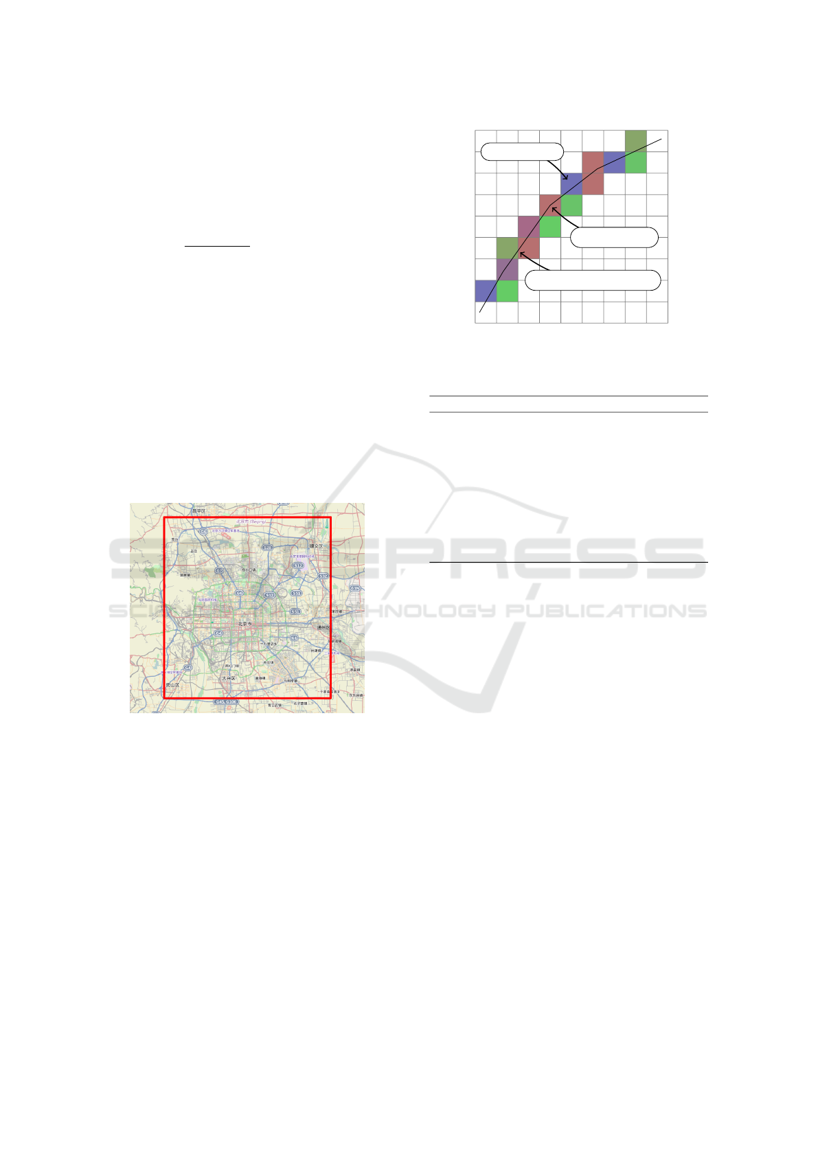
Figure 1: The experimental object region, which is a rect-

angle with side lengths of about 50 km in Beijing (map tiles

©OpenStreetMap contributors, CC BY-SA 2.0).

We chose data inside the area of central Beijing

shown in Figure 1, where observed GPS data were

not sparse. We generated trajectories by concatenat-

ing observations in chronological order whenever the

time gap between two consecutive observations was

10 s or less.

Next, we converted the original GeoLife trajectory

data into our trajectory form described in Section 2.1.

Figure 2 illustrates the method of conversion. We ﬁrst

split the area into cells with a width of 0.0006° of lon-

gitude and height of 0.0005° of latitude. Each cell g is

a rectangle with side lengths of about 50 m. An origi-

nal GeoLife trajectory is a sequence of spatiotemporal

points. We converted the trajectory by ﬁnding all the

•

Observed point

Linear-interpolated point

Converted cell

Figure 2: Trajectory conversion from the GeoLife dataset.

The color of a converted cell indicates the travel time within

it.

Table 1: Transportation modes and their priors.

mode mean speed ν [s] η a b

walk 1 km/h 180.0 10

−6

1 2

run 4 km/h 45.0 10

−6

1 2

bike 10 km/h 18.0 10

−6

1 2

bus 15 km/h 12.0 10

−6

1 2

taxi 20 km/h 9.0 10

−6

1 2

car 30 km/h 6.0 10

−6

1 2

subway 40 km/h 4.5 10

−6

1 2

train 60 km/h 3.0 10

−6

1 2

airplane 900 km/h 0.2 10

−6

1 2

cells through which it passes and calculating the trav-

eling time for each cell by linear interpolation. We

used 90% of the converted dataset for training and the

residual 10% of the data was used for the test. The

training dataset included nine-tenths of consecutive

trajectories for each user.

5.2 Model Parameter Estimation

We estimated the model parameters by MAP esti-

mation. There were 4,462,614 observations from

186,617 cells in the training dataset. We used prior

parameters for each mode, as shown in Table 1, which

we chose arbitrarily. The value of ν was determined

by dividing 50 m, which is equal to the length of a

side of a cell, by the mean travel speed we assumed

(Table 1). We also used prior and weight parameters:

α = β = 2.0, λ

= 0.5, λ

= 1.0.

We implemented the EM algorithm described

above using OpenMP for multiprocessing. The EM

algorithm has iterated the E step and the M step until

the improvement in log-likelihood fell below 0.01%.

The estimation was executed on our 32-core Xeon

computer. The EM algorithm was ﬁnished in nine it-

erations taking 11.3 s.

Figure 3 shows the estimated parameters; only

GPS Trajectory Data Enrichment based on a Latent Statistical Model

259

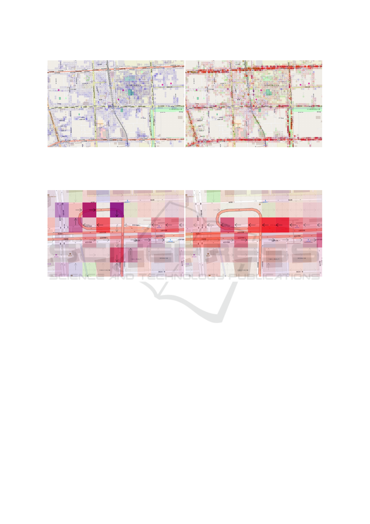
(a) Run. (b) Train.

BY-SA 2.0). Two of nine modes are shown because of space limitations. The color of a cell indicates the mean travel time

. Green represents short travel time (1.8 s), red is moderate travel time (3.6 s), and blue is long travel time (∞ s). The

opacity of a cell indicates θ

, the probability that the mode m is chosen in the cell g (opaquer is higher).

(a) Slower mode. (b) Faster mode.

Figure 4: Enlarged view of estimated model parameters around Zhongguancun exit on the North 4th Ring Road (expressway)

and θ

are shown in the same way as in

Figure 3, while arrows in a cell indicate φ

gmd

, the probability that the direction d is chosen with the mode m in the cell g

(bolder is higher).

two of nine modes are shown because of space limi-

tations. As can be seen, there are regional differences

of traveling mode tendencies: slower modes tend to

appear around local streets, while faster modes are

likely to appear on arteries or railways. Figure 4 is

an enlarged view, showing the differences in moving

direction and mean travel time between two different

modes. The moving direction is also learned, so that

a trajectory travels on the right side of wide roads and

that it takes different routes depending on the mode.

5.3 Interpolation and Traveling Mode

Estimation

We evaluated the performance of our interpolation

method. As our algorithm has high complexity, we

prepared a 3x5 dataset by collecting all subtrajecto-

ries that travel three cells along a north–south or

east–west direction and ﬁve cells along the orthog-

onal direction via the shortest path. For each sub-

trajectory in the 3x5 dataset, we estimated the inter-

mediate cells given its ﬁrst and last cells and its to-

tal travel time. The cardinality of the search space

was 2,410,616,376. The interpolation was ﬁnished

in 1 min for each subtrajectory using our 72-core

Xeon computer and the OpenMP technology. We

evaluated the interpolation performance by recall, i.e.,

the number of correctly interpolated cells divided by

the number of the total intermediate cells that actu-

ally included observation data of the original GeoLife

dataset.

In the test dataset, there were 8,276 subject sub-

trajectories and the recall was 78.8% (38,695 suc-

cess/49,092 cells). Although we did not conduct any

parameter tuning, more than three-quarters of the in-

terpolations were successful. There is an ample room

ICPRAM 2016 - International Conference on Pattern Recognition Applications and Methods

260

walk

run

bike

bus

taxi

car

subway

train

airplane

estimated mode

walk

run

bike

bus

taxi

car

subway

train

airplane

true mode

18 37

26 82

0 0 0 0 0 0 0 0 0

25 16 8 13 26 3

0 0

4 2

8 0

10 0

4 2

5 8 38 30 25

112

189 159

0 0 0 0 6 8 8

11 2 1

16 3 18

22 24

0 0 0 0 0 0 0 0 0

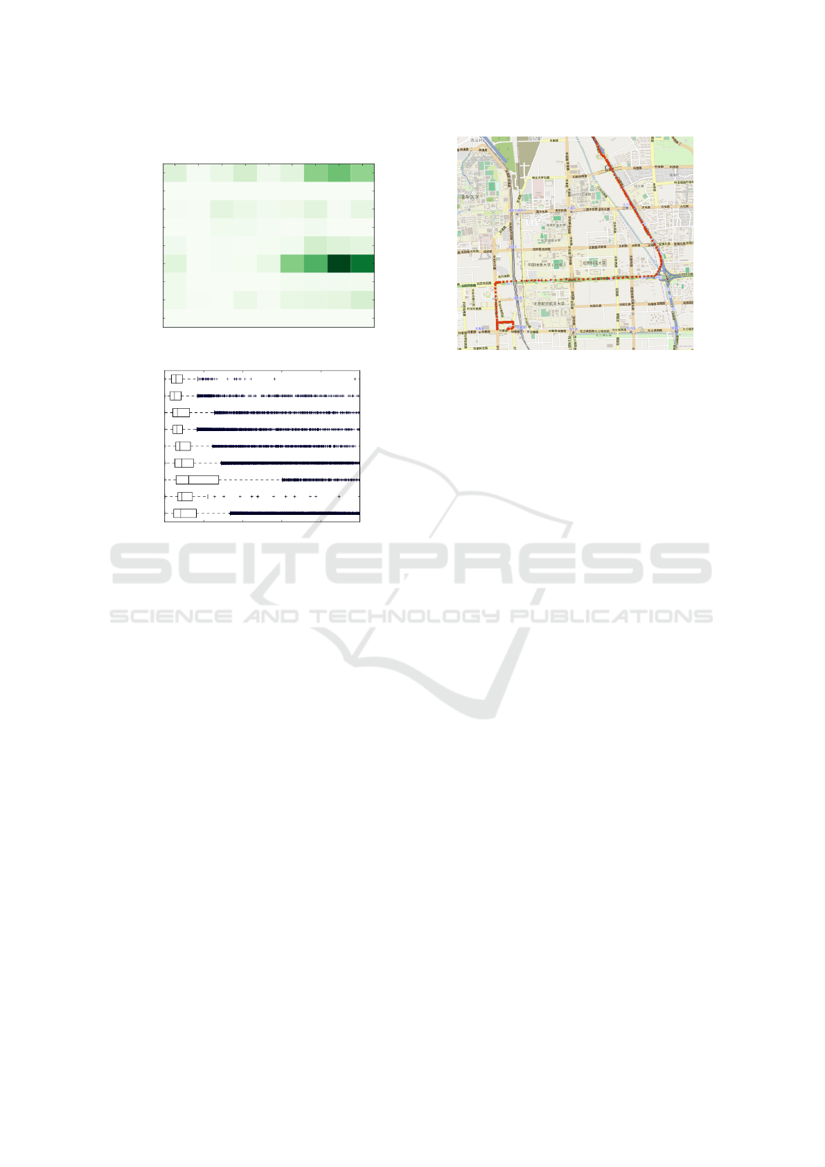
Figure 5: Confusion matrix of traveling mode estimation.

0 10 20 30 40 50

traveling time [sec]

walk

run

bike

bus

taxi

car

subway

train

airplane

Figure 6: Distribution of traveling time for each mode.

for improving performance by giving better priors and

weight parameters when the model is learned. On the

other hand, our interpolation method has high com-

plexity and is not scalable. Further work is being car-

ried out to improve the scalability of the algorithm.

Of the 3x5 subtrajectories in the test dataset, 309

have traveling mode labels. Our interpolation algo-

rithm estimated the traveling mode for each cell at

the same time as determining the cells. The accuracy

of the traveling mode was 12.9% (184 success/1,427

correctly interpolated cells). Figure 5 shows the con-

fusion matrix.

One possible reason for the poor accuracy of trav-

eling mode estimation is that the distribution of trav-

eling time was similar for all traveling modes. Fig-

ure 6 shows box plots of traveling time over the whole

dataset for each traveling mode. Here it can be seen

that the distributions of some modes, car and train for

example, were similar. This calls for further discus-

sion on feature selection. Another possible problem

is the labeling quality in the dataset. For example, a

GeoLife trajectory shown in Figure 7 was labeled as

“airplane” mode, but its movement was unnatural for

an airplane because it traveled along expressways, ar-

teries, and local streets. As the interpolation in this

experiment was conducted only in the spatial aspect,

Figure 7: A GeoLife trajectory labeled as “airplane” mode

it remains a challenge for future research to enrich tra-

jectories in the temporal aspect. Improving the perfor-

mance of traveling mode estimation would assist this

kind of trajectory enrichment.

6 CONCLUSION

We have studied the problem of GPS trajectory en-

richment, namely, interpolation and traveling mode

estimation. We developed a statistical model where

the traveling time and the moving direction depended

on both the location and the latent traveling mode,

whereas the mode also depended on the location. We

derived formulas to estimate the MAP parameters of

the model using GPS observation data which can in-

clude some observations with traveling mode labels.

Our method was applied to the GeoLife dataset. The

results showed that our model could describe the char-

acteristics of movements depending on location and

traveling mode and that more than three-quarters of

covered locations were correctly reproduced by inter-

polation at a ﬁne granularity. Future work will in-

clude the development of a more computationally ef-

ﬁcient interpolation algorithm, optimization of the set

of traveling modes, and feature selection.

ACKNOWLEDGEMENTS

This work was supported by CPS-IIP Project in the

research promotion program for national-level chal-

lenges “Research and development for the realization

of next-generation IT platforms” by the Ministry of

Education, Culture, Sports, Science and Technology,

Japan.

GPS Trajectory Data Enrichment based on a Latent Statistical Model

261

REFERENCES

Biau, G. and Fischer, A. (2012). Parameter selection

for principal curves. IEEE Trans. Inf. Theory,

58(3):1924–1939.

Bishop, C. M. (2006). Mixture Models and EM. In Pat-

tern Recognit. Mach. Learn., chapter 9, pages 423–

460. Springer, New York, NY, USA.

Brunsdon, C. (2007). Path estimation from GPS tracks. In

Proc. 9th Int. Conf. GeoComputation, Maynooth, Ire-

land.

Cao, L., Luo, J., Gallagher, A., Jin, X., Han, J., and Huang,

T. S. (2010). A worldwide tourism recommendation

system based on geotagged web photos. In 2010

IEEE Int. Conf. Acoust. Speech Signal Process., pages

2274–2277, Dallas, Texas, USA. IEEE.

Feng, T. and Timmermans, H. J. P. (2013). Map matching of

GPS data with Bayesian belief networks. Proc. East.

Asia Soc. Transp. Stud., 9.

Giannotti, F., Nanni, M., Pedreschi, D., and Pinelli, F.

(2007). Trajectory pattern mining. In Proc. 13th

ACM SIGKDD Int. Conf. Knowl. Discov. Data Min.

(KDD ’07), pages 330–339, San Jose, California,

USA. ACM.

Goh, C. Y., Dauwels, J., Mitrovic, N., Asif, M. T., Oran,

A., and Jaillet, P. (2012). Online map-matching based

on Hidden Markov model for real-time trafﬁc sensing

applications. In 15th Int. IEEE Conf. Intell. Transp.

Syst., pages 776 – 781, Anchorage, Alaska, USA.

IEEE.

onroos, S.-A., Virpioja, S., Smit, P., and Kurimo,

M. (2014). Morfessor FlatCat: An HMM-based

method for unsupervised and semi-supervised learn-

ing of morphology. In Proc. COLING 2014, 25th Int.

Conf. Comput. Linguist. Tech. Pap., pages 1177–1185,

Dublin, Ireland.

Hao, P., Boriboonsomsin, K., Wu, G., and Barth, M. (2014).

Probabilistic model for estimating vehicle trajectories

using sparse mobile sensor data. In 2014 IEEE 17th

Int. Conf. Intell. Transp. Syst. (ITSC ’14), pages 1363–

1368, Qingdao, China. IEEE.

Karagiorgou, S. and Pfoser, D. (2012). On vehicle tracking

data-based road network generation. In Proc. 20th Int.

Conf. Adv. Geogr. Inf. Syst. (SIGSPATIAL ’12), pages

89–98, Redondo Beach, California. ACM.

Kinoshita, A., Takasu, A., and Adachi, J. (2015). Real-time

trafﬁc incident detection using a probabilistic topic

model. Inf. Syst., 54:169–188.

Monreale, A., Pinelli, F., Trasarti, R., and Giannotti, F.

(2009). WhereNext: A location predictor on trajectory

pattern mining. In Proc. 15th ACM SIGKDD Int. Conf.

Knowl. Discov. Data Min. (KDD ’09), pages 637–646,

Paris, France. ACM.

Sankararaman, S., Agarwal, P. K., Mølhave, T., Pan, J.,

and Boedihardjo, A. P. (2013). Model-driven match-

ing and segmentation of trajectories. In Proc. 21st

ACM SIGSPATIAL Int. Conf. Adv. Geogr. Inf. Syst.

(SIGSPATIAL ’13), pages 234–243, Orlando, Florida.

ACM.

Schnitzler, F., Artikis, A., Weidlich, M., Boutsis, I.,

Liebig, T., Piatkowski, N., Bockermann, C., Morik,

K., Kalogeraki, V., Marecek, J., Gal, A., Mannor,

S., Kinane, D., and Gunopulos, D. (2014). Het-

erogeneous stream processing and crowdsourcing for

trafﬁc monitoring: Highlights. In Proc. Eur. Conf.

Mach. Learn. Princ. Pract. Knowl. Discov. Databases

(ECML PKDD ’14), pages 520–523, Nancy, France.

Springer Berlin Heidelberg.

Wang, Y., Zheng, Y., and Xue, Y. (2014). Travel time esti-

mation of a path using sparse trajectories. In Proc.

20th ACM SIGKDD Int. Conf. Knowl. Discov. data

Min. (KDD ’14), pages 25–34, New York, New York,

USA. ACM.

Wei, H., Wang, Y., Forman, G., Zhu, Y., and Guan, H.

(2012). Fast Viterbi map matching with tunable

weight functions. In Proc. 20th Int. Conf. Adv. Geogr.

Inf. Syst. (SIGSPATIAL ’12), pages 613–616, Redondo

Beach, California. ACM.

Yang, Q., Wu, G., Boriboonsomsin, K., and Barth, M.

(2013). Arterial roadway travel time distribution es-

timation and vehicle movement classiﬁcation using a

modiﬁed Gaussian mixture model. In 16th Int. IEEE

Conf. Intell. Transp. Syst. (ITSC ’13), pages 681–685,

The Hague, The Netherlands. IEEE.

Yang, W.-S., Cheng, H.-C., and Dia, J.-B. (2008). A

location-aware recommender system for mobile shop-

ping environments. Expert Syst. Appl., 34(1):437–

445.

Yu, S.-Z. and Kobayashi, H. (2003). A hidden semi-Markov

model with missing data and multiple observation se-

quences for mobility tracking. Signal Processing,

83:235–250.

Zheng, Y., Chen, Y., Li, Q., Xie, X., and Ma, W.-Y. (2010a).

Understanding transportation modes based on GPS

data for web applications. ACM Trans. Web, 4(1):1:1–

1:36.

Zheng, Y., Li, Q., Chen, Y., Xie, X., and Ma, W.-Y. (2008).

Understanding mobility based on GPS data. In Proc.

10th Int. Conf. Ubiquitous Comput. (UbiComp ’08),

pages 312–321, Seoul, Korea. ACM.

Zheng, Y., Xie, X., and Ma, W.-Y. (2010b). GeoLife: A

collaborative social networking service among user,

location and trajectory. Bull. Tech. Comm. Data Eng.,

33(2):32–39.

Zheng, Y., Zhang, L., Xie, X., and Ma, W.-Y. (2009). Min-

ing interesting locations and travel sequences from

GPS trajectories. In Proc. 18th Int. Conf. World Wide

Web (WWW ’09), pages 791–800, Madrid, Spain.

ACM.

Zhu, X. and Goldberg, A. B. (2009). Introduction to Semi-

Supervised Learning. Morgan & Claypool.

ICPRAM 2016 - International Conference on Pattern Recognition Applications and Methods

262