
Fixed-sequence Single Machine Scheduling and Outbound Delivery
Problems
Azeddine Cheref
1,2,3
, Alessandro Agnetis
4
, Christian Artigues
2,3
and Jean-Charles Billaut
1
1
Universit
´
e Franc¸ois-Rabelais Tours / CNRS, 64 av. J. Portalis, 37200 Tours, France
2
CNRS, LAAS, 7 Avenue du Colonel Roche, F-31400 Toulouse, France
3
Univ. de Toulouse, LAAS, F-31400 Toulouse, France
4
Dipartimento di Ingegneria dell’Informazione, Universit
´
a degli Studi di Siena, via Roma 56, 53100 Siena, Italy
Keywords:
Scheduling, Batching and Delivery, Computational Complexity, Dynamic Programming.
Abstract:
In this paper, we study an integrated production an outbound delivery scheduling problem with a predefined
sequence. The manufacturer has to process a set of jobs on a single machine and deliver them in batches to
multiple customers. A single vehicle with limited capacity is used for the delivery. Each job has a processing
time and a specific customer location. Starting from the manufacturer location, the vehicle delivers a set of
jobs which constitute a batch by taking into account the transportation times. Since the production sequence
and delivery sequence are fixed and identical, the problem consists in deciding the composition of batches.
We prove that for any regular sum-type objective function of the delivery times, the problem in NP-hard in the
ordinary sense and can be solved in pseudopolynomial time. A dynamic programming algorithm is proposed.
1 INTRODUCTION
This paper deals with a model for coordinating pro-
duction and delivery schedules. In many produc-
tion systems, finished products are delivered from the
factory to multiple customer locations, warehouses,
or distribution centers by delivery vehicles. An in-
creasing amount of research has been devoted, dur-
ing the last twenty years, to devise integrated models
for production and distribution. These models have
been largely analyzed and reviewed by (Chen, 2010),
who proposed a detailed classification scheme. The
models reflect the variety of issues, including sys-
tems structure, vehicle/transportation system charac-
teristics, delivery modes, various types of time con-
straints. In the large majority of the models in the
literature, the coordination of production and distri-
bution is achieved through the creation of batches,
i.e., several parts are shipped together and delivered
to their respective destinations during a single trip.
When forming batches, one must therefore take into
account both production information (such as pro-
cessing time, release dates etc) and delivery informa-
tion (such as customer location, time windows etc).
Most of the models presented in the literature explic-
itly take into account transportation times to reach the
customers’ location, but there are no proper routing
decisions, since the number of distinct customers is
typically very small. Hence, the focus of the analysis
is often on scheduling and batching.
Many models consider delivery as a separate step
after production, but do not model it in details, e.g. as-
suming that a sufficiently large number of vehicles is
available to deliver the products at any time (Chen and
Lee, 2008) (Agnetis et al., 2014) (Fan et al., 2015), or
assuming that there is a single customer. In (Chang
and Lee, 2004) the jobs have a certain size and the ca-
pacity of a vehicle is a physical space available, and
jobs have to be delivered to a unique customer. NP-
hardness results are given as well as heuristic algo-
rithms with performance guarantee. In (Li and Ou,
2005) and (Wang and Cheng, 2009), delivery con-
cerns the materials as well as finished jobs which must
be transported to a single warehouse. The objective
is to minimize the delivery time of the job delivered
last to this customer. Li and Ou propose a polynomial
time algorithm when the production sequence is fixed.
In the literature, delivery can also be modeled as a
delay after the production completion time. Fan, Lu
and Liu (Fan et al., 2015) consider the join problem of
scheduling and routing with availability constraints of
the machine. The delivery is performed by an unlim-
ited number of uncapacitated vehicles and the objec-
tive is to minimize the total delivery time and total de-
Cheref, A., Agnetis, A., Artigues, C. and Billaut , J-C.
Fixed-sequence Single Machine Scheduling and Outbound Delivery Problems.
DOI: 10.5220/0005701201450151
In Proceedings of 5th the International Conference on Operations Research and Enterprise Systems (ICORES 2016), pages 145-151
ISBN: 978-989-758-171-7
Copyright
c
2016 by SCITEPRESS – Science and Technology Publications, Lda. All rights reserved
145

livery cost. Depending on the problem they consider,
the authors propose polynomial time algorithms, an
algorithm with guaranteed performance and a poly-
nomial time approximation scheme.
In the paper by (Li et al., 2005), a single vehicle
is used for delivery, and hence the vehicle schedule
has to be synchronized with production and batching
decisions. In particular, one must also take account
of the time that the vehicle will take to deliver a cer-
tain batch of products, and that it will take to be back
at the manufacturing facility. (Li et al., 2005) ana-
lyze the joint problem of production sequencing and
batch formation, in order to minimize total delivery
time, given that delivery is performed by a single ve-
hicle. Total delivery time is a meaningful indicator
of the overall efficiency of the delivery process. They
show that in general the problem is NP-hard, and then
give polynomial time algorithms for the problem with
a fixed number of distinct destinations. In (Tsirim-
pas et al., 2008), the authors consider that all the jobs
are ready for the delivery at the beginning of the time
horizon (no scheduling problem here). The delivery
is performed by a single capacitated vehicle and the
sequence of delivery is predefined. The objective is
to minimize the total travel time and the authors pro-
pose polynomial time algorithms. In (Chen and Lee,
2008), the authors consider the problem with a single
machine where finished jobs must be transported by
an unlimited number of vehicles. There is no vehicle
routing problem, since the vehicle delivers in one trip
only jobs delivered at the same destination.
Using the terminology of (Chen, 2010), the mod-
els presented in this paper concern batch delivery with
routing, i.e., orders going to different customers can
be delivered together in the same shipment (batch).
A distinctive feature of the problems we address
here is that the jobs must be delivered in the same
order in which they are produced (we can simply as-
sume that the delivery sequence is fixed and in this
case, there is always an optimal production sequence
which is the same as the delivery sequence). Ex-
amples of situations in which the customer sequence
is fixed are reported by (Armstrong et al., 2008),
(Viergutz and Knust, 2014) and include a fixed se-
quence of customers and a single round trip for the
delivery, as well as the objective is to maximize the
total demand without violating the product lifespan.
This problem is proved NP-hard by (Armstrong et al.,
2008). In (Lent
´
e and Kergosien, 2014), the authors
consider that the production sequence is fixed as well
as the delivery sequence. The authors search for a
batching of jobs minimizing the makespan, the maxi-
mum lateness and the number of tardy jobs. The prob-
lems are modeled by a graph and polynomial time al-
gorithms are proposed for these objective functions.
In this paper, we will mainly focus on the problem
of deciding how to form batches with a given pro-
duction sequence (problem P1). We completely char-
acterize the complexity of Problem P1, showing that
when the objective function is to minimize the total
delivery time it is NP-hard in the ordinary sense, and
that it can be solved in pseudopolynomial time for any
sum-type function of the delivery times.
The paper is organized as follows. In Section 2
we present the problem formally and show that the
problem is NP-hard when Z is the total delivery time,
and that it can be solved in pseudopolynomial time
when Z is any sum-type objective function. Finally,
some conclusions and future research directions are
presented in Section 4.
2 PROBLEM DEFINITION AND
COMPLEXITY
2.1 Problem Definition and Notation
The problem considered in this paper can be de-
scribed as follows. A set of n jobs is given and
their production sequence is known. Each job J
j
,
j = 1, ...,n, requires a certain processing time p
j
on
a single machine, and must be delivered to a certain
location site. We assume w.l.o.g. that the production
sequence is (J
1
,J
2
,...,J
n
). For the sake of simplicity,
when it does not create confusion, we use j to refer to
the destination of job J
j
. We denote by t
i, j
the trans-
portation time from destination i to destination j. For
analogy with vehicle routing problems, we refer to the
manufacturer’s location as the depot. We use M to de-
note the depot (manufacturer), hence t
M,j
= t
j,M
is the
transportation time between the depot and destination
j. Unless otherwise specified, we assume that trans-
portation times are symmetric and satisfy the triangle
inequality.
Deliveries are carried out by a single vehicle. The
vehicle loads a certain number of jobs which have
been processed and departs towards the correspond-
ing destinations. Thereafter, it returns to the depot,
hence completing a round trip. The set of jobs de-
livered during a single round trip constitutes a batch.
The capacity c of the vehicle is the maximum num-
ber of jobs it can load and hence deliver in a round
trip. The jobs must be delivered in the order in which
they are produced, hence the production sequence
also specifies the sequence in which the customers
have to be reached.
The problem consists in deciding a partition of
ICORES 2016 - 5th International Conference on Operations Research and Enterprise Systems
146

all jobs into batches, i.e., a batching scheme. Each
batch will be routed according to the manufacturing
sequence. In general, the performance of the sys-
tem depends on all the concurrent decisions: produc-
tion scheduling, batching and vehicle routing. This
requires therefore an integrated model, allowing the
coordination of all these aspects. A solution to our
problem with fixed sequence, is the specification of a
batching scheme. Given a solution, we denote by C
j
the completion time of job J
j
on the single machine,
which is also the time at which the job is released for
delivery, i.e., the batch including job J
j
cannot start
before C
j
. We denote by D
j
the delivery time of J
j
,
i.e., the time at which the job J
j
is delivered at its des-
tination. The performance measures we consider in
this paper depend on such delivery times. In particu-
lar, denoting with Z the performance measure, in this
paper we consider:
• the total delivery time, i.e., Z =
∑
n
j=1
D
j
• a general sum-type performance index, i.e., Z =
∑
n
j=1
f
j
(D
j
), where f
j
(D
j
) is a general, nonde-
creasing function of D
j
, j = 1,...,n.
Note that the latter case includes total (weighted)
delivery time, total (weighted) tardiness, etc.
We consider the following problem:
Problem P1(Z). Given n jobs of length p
j
, j =
1,... ,n, transportation times t
i, j
for all i, j, and a se-
quence σ, find a batching scheme B such that Z is
minimized.
2.2 Complexity
Since the production sequence is given, and since
jobs are delivered to the respective customers in the
same given order, we assume that the job sequence
is σ = (J
1
,J
2
,...,J
n
). Only travel times t
j, j+1
are rel-
evant, as well as times t
j,M
= t
M,j
, representing the
travel time between customer j and the manufacturer
or vice-versa.
Let us first consider the problem when the objec-
tive to minimize is the total delivery time, i.e., prob-
lem P1(
∑
n
j=1
D
j
). For our purposes, we introduce the
following problem.
EVEN-ODD PARTITION (EOP). A set of n pairs
of positive integers (a
1
,b
1
),(a
2
,b
2
),... , (a
n
,b
n
) is
given, in which, for each i, a
i
> b
i
. Letting K =
∑
n
i=1
(a
i
+ b
i
), is there a partition (S,
¯
S) of the index
set I = {1,2,... ,n} such that
∑
i∈S
a
i
+
∑
i∈
¯
S
b
i
= K/2? (1)
EOP is NP-hard in the ordinary sense (Garey et al.,
1988). In the following, we will actually use the fol-
lowing slightly modified version of the problem.
MODIFIED EVEN-ODD PARTITION (MEOP). A
set of n pairs of positive integers (a
1
,b
1
),(a
2
,b
2
),
..., (a
n
,b
n
) is given, in which, for each i, a
i
> b
i
. Let-
ting Q =
∑
n
i=1
(a
i
−b
i
), is there a partition (S,
¯
S) of the
index set I = {1,2,. ..,n} such that
∑
i∈S
(a
i
− b
i
) = Q/2? (2)
Note that the two problems are indeed equiva-
lent. In fact, suppose that EOP has a partition (S,
¯
S).
The corresponding instance of MEOP also admits the
same partition. In fact, subtracting
∑
n
i=1
b
i
=
∑
i∈S
b
i
+
∑
i∈
¯
S
b
i
from both sides of (1), one obtains
∑
i∈S
(a
i
− b
i
) = K/2 −
n
∑
i=1
b
i
(3)
Now, from the definitions of K and Q it turns out that
Q = K − 2
n
∑
i=1
b
i
and hence (3) is indeed (2). We next show the follow-
ing result.
Theorem 2.1. P1(
∑
n
j=1
D
j
) is NP-hard.
Proof. The problem is obviously in NP. Given an in-
stance of MEOP, we build an instance of P1 as fol-
lows. There are 3n + 3 jobs. The processing times of
the jobs are defined as follows:
• p
1
= p
2
= p
3
= 0.
• for each i = 0, 1, ..., n − 1, one has
– p
3i+1
= p
3i+2
= 1,
– p
3i+3
= 4x
i
+ b
i
− 2.
• p
3n+1
= 4x
n
+ b
n
+ Q/2.
• p
3n+2
= p
3n+3
= 0,
where the x
i
are defined by
x
i
= (3a
i
−2b
i
+3(n −i)(a
i
−b
i
))/2 ∀ i = 1 . . .n (4)
and x
n+1
= 0.
In the following, we refer to the set of jobs
(J
3i+1
,J
3i+2
,J
3i+3
), i = 0,..., n, as the triple T
i+1
.
For what concerns the travel times, we let:
• for each i = 0, 1, ..., n − 1, one has
– t
M,3i+1
= t
3i+1,M
= t
M,3i+2
= t
3i+2,M
= t
M,3i+3
=
t
3i+3,M
= x
i+1
,
– t
3i+1,3i+2
= a
i+1
,
– t
3i+2,3i+3
= b
i+1
,
– t
3i+3,3i+4
= x
i+1
+ x
i+2
.
• t
M,3n+1
= t
3n+1,M
= t
M,3n+2
= t
3n+2,M
= t
M,3n+3
=
0.
• t
3n+1,3n+2
= t
3n+2,3n+3
= 0.
Fixed-sequence Single Machine Scheduling and Outbound Delivery Problems
147

Finally, vehicle capacity is c = 2. The problem
consists in determining whether a solution exists such
that the total delivery time does not exceed
f
∗
=
n
∑
i=1
(3C
3i
+7x
i
+b
i
)+C
3n+1
+C
3n+2
+C
3n+3
−Q/2.
(5)
For shortness, we call feasible a schedule satisfy-
ing (5). The proof has the following scheme.
1. We first establish that if a feasible schedule exists,
then there is one having a certain structure, called
triple-oriented,
2. We analyze some properties of this structure,
3. We show that a triple-oriented schedule of value
f
∗
exists if and only if EOP is a yes-instance.
Lemma 2.2. If a feasible schedule exists, then there
exists one satisfying the following property: for all
i = 1,.. .,n+1, jobs J
3i
and J
3i+1
are NOT in the same
batch.
Proof. Suppose that a feasible schedule exists in
which, for a certain i (1 ≤ i ≤ n), jobs J
3i
and J
3i+1
are in the same batch. Since c = 2, the batch contains
no other job. As a consequence, after delivering J
3i+1
,
the vehicle must go back to M in order to load the next
jobs and start a new trip. If we denote by τ the start
time of the round trip of jobs J
3i
and J
3i+1
, job J
3i
is
delivered at time D
3i
= τ + t
M,3i
and job J
3i+1
is de-
livered at time D
3i+1
= τ + t
M,3i
+ t
3i,3i+1
. Therefore
we have D
3i
= τ + x
i
and D
3i+1
= τ + x
i
+ (x
i
+ x
i+1
).
The vehicle is back at M at time τ + 2x
i
+2x
i+1
. Now,
if we replace this batch with two batches of one job
each, the delivery times of both jobs as well as the
time at which the vehicle is back at M are unchanged.
Therefore, there is an equivalent solution where J
3i
and J
3i+1
are not in the same batch.
We call triple-oriented a schedule satisfying
Lemma 2.2. The reason of this name is that
the schedule is decomposed according to triples.
More precisely, since c = 2, for each triple T
i+1
=
(J
3i+1
,J
3i+2
,J
3i+3
), i = 0,. ..,n − 1, there are exactly
two batches, and only two possibilities, namely:
• either the first batch is {J
3i+1
,J
3i+2
} and the sec-
ond is {J
3i+3
},
• or the first batch is {J
3i+1
} and the second is
{J
3i+2
,J
3i+3
}.
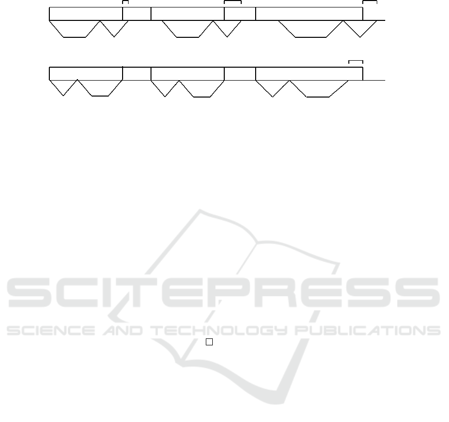
We call these two possibilities option A and option
B respectively (see Fig. 1). Namely, let us view option
B as the Base option, and A as a variant to it.
Round trip length. Letting M
A
i
and M
B
i
denote the
round trip length of the jobs of T
i
in the two cases.
One has:
M
A
i
= 4x
i
+ a
i
(6)
M
B
i
= 4x
i
+ b
i
(7)
Since a
i
> b
i
, option A implies a longer round trip
length than the Base option. The difference between
the two lengths M
A
i
− M
B
i
is precisely equal to a
i
− b
i
.
Lemma 2.3. In any triple-oriented schedule, the ve-
hicle is never idle, except possibly before loading
J
3n+1
.
Proof. The lemma is proved by an induction argu-
ment. Let consider the first triple T
1
. The vehicle
starts at time 0 (to deliver batch {J
1
} or {J
1
,J
2
}), and
is back at time 4x
1
+ b
1
or at time 4x
1
+ a
1
. The
production completion time of the jobs of T
2
is pre-
cisely equal to C
6
=
∑
6
j=1
p
j
= 1 + 1 +4x
1
+b
1
−2 =
4x
1
+b
1
. Therefore, the vehicle can immediately start
the delivery of the jobs of T
2
. For the same reasons,
the delivery time of the jobs of T
i
cannot be smaller
than the duration of the processing of the jobs of T
i+1
,
and the vehicle will be able to start immediately the
delivery of the jobs of T
i+1
. This reasoning stops for
the last triple T
n+1
because the duration of J
3n+1
is
particular.
In view of Lemma 2.3, one can compute the total
delivery time in the Base scenario, i.e., when option
B is always chosen. From (7), one has that the vehicle
always returns to M exactly at time C
3i
. Therefore, the
last time the vehicle arrives at M (before delivering
the jobs of T
n+1
) is C
3n
+ 4x
n
+ b
n
. Because of the
definition of p
3n+1
, and because J
3n+1
starts at time
C
3n
, this time is equal to C
3n+3
− Q/2. In this case,
the vehicle will stay idle from C
3n+1
− Q/2 to C
3n+1
,
when job J
3n+1
can be finally loaded (see Fig.2) and
delivered (the two reminder jobs have a duration of 0
and travel times equal to 0). Hence, we have:
f
BASE
=
n
∑
i=1
(3C
3i
+ 7x
i
+ b
i
) +C
3n+1
+C
3n+2
+C
3n+3
(8)
Contribution to total delivery time. Before com-
puting the contribution of a certain triple to the to-
tal delivery time, let us consider schedules in which
the last three jobs J
3n+1
, J
3n+2
and J
3n+3
start exactly
their transportation at their release time, i.e., at time
C
3n+1
= C
3n+2
= C
3n+3
(options A and B are equiva-
lent). Let us call regular a schedule in which such a
condition holds.
Expression (8) refers to the scenario in which for
all triples, the option B is chosen. We want now to
compute the objective function of an arbitrary solu-
tion. Let us first consider the contribution of triple T
i
to the objective function in the Base schedule, i.e., as-
suming that the delivery of T
i
started at time C
3i
, and
ICORES 2016 - 5th International Conference on Operations Research and Enterprise Systems
148

3(i-1)+1 3(i-1)+2 3(i-1)+3
b
i
3(i-1)+1 3(i-1)+2 3(i-1)+3
a
i
3i+1 3i+2 3i+3
3i+1 3i+2 3i+3
option A
option B
a
i
− b
i
Figure 1: Round trips with options A and B.
...
3(i-1)+1 3(i-1)+2 3(i-1)+3
b
i
3i+1 3i+2 3i+3
x
i
x
i
x
i
x
i
T
i+1
T
i
Figure 2: The base schedule (i.e., B is always chosen).
let us denote such piece of contribution as T DT
A
i
and
T DT
B
i
in the two cases. One has:
T DT
A
i
= (C
3i
+ x
i
) + (C
3i
+ x
i
+ a
i
) + (C
3i
+ 3x
i
+ a
i
)
= 3C
3i
+ 5x
i
+ 2a
i
(9)
T DT
B
i
= (C
3i
+ x
i
) + (C
3i
+ 3x
i
) + (C
3i
+ 3x
i
+ b
i
)
= 3C
3i
+ 7x
i
+ b
i
(10)
Note that
T DT
B
i
− T DT
A
i
= 2x
i
+ b
i
− 2a
i
= (3a
i
− 2b
i
+ 3(n − i)(a
i
− b
i
)) + b
i
− 2a
i
= a
i
− b
i
+ 3(n − i)(a
i
− b
i
) (11)
which is positive, remembering that a
i
> b
i
. This
means that choosing option A over B brings a bene-
fit in terms of total delivery time. However, such fa-
vorable situation for option A is mitigated by the fact
that, with option A, one has a longer round trip time
than with option B, by the amount (a
i
−b
i
) (Fig.3). In
a regular schedule, such increased round trip time will
be ”paid” by all subsequent jobs, except the last jobs
J
3n+1
, J
3n+2
and J
3n+3
. Hence, in a regular schedule
the total effect (in favor of option B) on the subse-
quent jobs of choosing option A for T
i
is given by
3(n − i)(a
i
− b
i
) (12)
In conclusion, the net benefit of choosing option
A over B for T
i
in terms of objective function value
is obtained subtracting (12) from (11), and in view of
the definition of x
i
(4), one has therefore that
NetBene f it
i
= (2x
i
+ b
i
− 2a
i
) − 3(n − i)(a
i
− b
i
)
= a
i
− b
i
(13)
...
a
i
− b
i
3(i-1)+1 3(i-1)+2 3(i-1)+3
a
i
x
i
x
i
x
i
x
i
T
i+1
T
i
3i+1 3i+2 3i+3
Figure 3: T
i
is the first triple choosing option A.
In conclusion, it turns out that, when A is chosen
over the Base option, one has a larger round trip time,
by (a
i
− b
i
), but also a smaller contribution to total
delivery time (also by the amount (a
i
− b
i
))(see Fig.
4). So, given any regular triple-oriented schedule in
which the last three jobs depart at their completion
time, let T
A
be the set of triples for which the option
A is chosen. Then, from the above considerations, the
value f of the objective function is given by
f = f
BASE
−
∑
i∈T
A
(a
i
− b
i
) (14)
On the other hand, the time at which the vehicle re-
turns to M before loading the last three jobs (J
3n+1
,
J
3n+2
and J
3n+3
) is given by
C
3n
+ 4x
n
+ b
n
+
∑
i∈T
A
(a
i
− b
i
) (15)
Now, in a regular schedule job J
3n+1
(and also
J
3n+2
and J
3n+3
) starts at time C
3n+1
= C
3n
+ 4x
n
+
b
n
+ Q/2. Hence, from (15), in a regular schedule, it
must hold:
∑
i∈T
A
(a
i
− b
i
) ≤ Q/2
On the other hand, comparing (5), (8) it turns out
that
f
∗
= f
BASE
− Q/2
and hence, from (14), a regular schedule is feasi-
ble precisely if a subset T
A
of indices exists such that
∑
i∈T
(a
i
−b
i
) = Q/2, i.e., if and only if a feasible par-
tition exists in the instance of EOP. To conclude the
proof, it is left to show that f
∗
can be attained only by
a regular schedule. In fact, if a schedule is not regular,
Fixed-sequence Single Machine Scheduling and Outbound Delivery Problems
149
.... ....
T
i+1
3(i-1)+1 3(i-1)+2
3i
b
i
.... ....
T
i+1
∑
i
j=1
a
j
− b
j
3(i-1)+1 3(i-1)+2
3i
a
i
T
2
1 2
3
a
1
T
2
1 2
3
b
1
3n+1, 3n+2, 3n+3
3(n-1)+1 3(n-1)+2
3n
a
n
Q/2
3n+1, 3n+2, 3n+3
3(n-1)+1 3(n-1)+2
3n
b
n
Q/2
a
1
− b
1
Figure 4: Round trips with option A only and option B only.
the departure time of the last batch is delayed by the
amount (
∑
i∈T
A
(a
i
− b
i
) − Q/2) with respect to C
3n+1
.
As a consequence, the expression of f in (14) must
be modified to take account of such delay of the last
three jobs, i.e. it comes
f = f
BASE
−
∑
i∈T
A
(a
i
− b
i
) + 3(
∑
i∈T
A
(a
i
− b
i
) − Q/2)
= f
BASE
+ 2
∑
i∈T
A
(a
i
− b
i
) − 3Q/2 (16)
Since, in a nonregular schedule,
∑
i∈T
A
(a
i
− b
i
) > Q/2,
from (16) one has
f > f
BASE
+ Q − 3Q/2 = f
BASE
− Q/2
and hence it cannot be feasible.
3 PSEUDOPOLYNOMIAL TIME
ALGORITHM FOR P1(
∑
j
f
j
(D
j
))
Theorem 2.1 implies that no optimal polynomial time
algorithm can be found for P1(
∑
n
j=1
D
j
), and hence
for more general objective functions, unless P=NP.
In what follows, we show that P1(
∑
j
f
j
(D
j
)) can be
solved in pseudopolynomial time, hence settling the
complexity status of P1.
In what follows we denote by {i, j} the batch con-
sisting of jobs J
i
,... ,J
j
. As usual, C
j
is the com-
pletion time of job J
j
(known because σ is known),
and hence the release time for delivery. We denote by
M(i, j) the duration of the round trip of batch {i, j},
and, if the batch starts at time t, we call K(i, j,t) its
contribution to the objective function. Also, we as-
sume that at the beginning, the vehicle is at the man-
ufacturing location.
We denote by F(i, j,t) the value of the optimal
solution of the problem restricted to the first j jobs,
in which the first job of the last batch is J
i
, and such
that the batch starts at time t. Then, F(i, j,t) can be
computed by means of a simple recursive formula. In
the optimal solution of the subproblem, if the second
last batch is {p,i − 1}, and if it starts at time s, then
we have:
F(i, j,t) = F(p,i − 1,s) + K(i, j,t)
Note that, if the vehicle starts at time s, it must be
back before or at time t, i.e., the following constraint
must hold:
C
i−1
≤ s ≤ t − M(p,i − 1)
In conclusion, the problem is solved by means of:
F(i, j,t) = min
max(i−c,1)≤p≤i−1
C
i−1
≤s≤t−M(p,i−1)
{F(p,i−1, s)}+K(i, j,t)
(17)
Let T be an upper bound on the latest possible de-
parture time for the last batch. As long as the triangle
inequality holds, this is given, for instance, by:
T = max
max
1≤i≤n−1
{C
i
+ 2
n−1
∑
h=i
t
hM
},C
n
!
The optimal solution is given by:
z
∗
= min
n−c+1≤i≤n,C
n
≤t≤T
F(i,n,t)
(18)
A few boundary conditions must be imposed:
F(i, j,t) = +∞ for all j < i (19)
F(1, j,t) = K(1, j,t) for all j,t (20)
Condition (19) is obvious. Condition (20) allows
to initialize the algorithm.
Let us turn to complexity. First, consider the com-
putation of values M(i, j) and K(i, j,t). Both can be
simply computed adding the contribution of the next
job in the batch either to the round trip time (for
M(i, j)) or to the objective function (for K(i, j,t)).
More precisely, the delivery time d
h
of job J
h
with
ICORES 2016 - 5th International Conference on Operations Research and Enterprise Systems
150

respect to the departure time of the batch is simply
given by:
d
h
=
d
h−1
+t
h−1,h
, if i < h ≤ j
t
M,h
, if h = i (in this case the
vehicle starts from M)
Hence, M(i, j) is simply given by d
j
+ t
j,M
. Note
that M(i, j +1) = M(i, j) −t
j,M
+t
j, j+1
+t
j+1,M
. This
means that all M(i, j) can be computed in O(nc) as-
suming j ≤ i + c − 1. Similarly, if batch {i, j} starts
indeed at time t, the contribution of job J
h
to the ob-
jective function is given by:
f
h
(t + d
h
),∀i ≤ h ≤ j
Clearly, K(i, j,t) is given by
∑
j
h=i
f
h
(t + d
h
).
Again, assuming that f
j
(·) can be computed in con-
stant time, note that d
j+1
= d
j
+ t
j, j+1
and K(i, j +
1,t) = K(i, j,t) + f
j+1
(d
j+1
). So, all values K(i, j,t)
can be computed in O(ncT ).
Once all values M(i, j) and K(i, j,t) are known,
one can compute formula (17) for all feasible triples
(i, j,t). Each such computation requires comparing
nT values. Finally, O(cT ) values are compared to
find the optimal solution. Since the feasible triples are
O(ncT ), the computation of all values F(i, j,t) clearly
dominates the other phases, and the following result
is proved.
Theorem 3.1. Problem P1(
∑
j
f
j
(D
j
)) can be solved
in pseudopolynomial time in O(nc
2
T
2
).
4 CONCLUSION AND FUTURE
RESEARCH DIRECTIONS
The problem treated in this paper takes place in a Sup-
ply Chain environment, where a manufacturer (mod-
eled as a single machine) has to organize the delivery
of the items (performed by a single capacitated ve-
hicle). The sequence of production is given, and is
supposed to be the same as the sequence of delivery.
The problem is to form batches of jobs, so that the
total delivery time is minimised. We prove that the
problem is NP-hard for a capacity equal to 2, and a
pseudopolynomial time dynamic programming algo-
rithm is proposed.
We are going to investigate the case where the se-
quence is not fixed. Several polynomial cases can
be proposed as well as dynamic programming algo-
rithms for non-polynomial cases.
ACKNOWLEDGEMENTS
This work was supported by the financial sup-
port of the ANR ATHENA project, grant ANR-13-
BS02-0006 of the French Agence Nationale de la
Recherche.
REFERENCES
Agnetis, A., Aloulou, M. A., and Fu, L.-L. (2014). Co-
ordination of production and interstage batch deliv-
ery with outsourced distribution. European Journal
of Operational Research, 238(1):130 – 142.
Armstrong, R., Gao, S., and Lei, L. (2008). A zero-
inventory production and distribution problem with a
fixed customer sequence. Annals of Operations Re-
search, 159(1):395–414.
Chang, Y.-C. and Lee, C.-Y. (2004). Machine scheduling
with job delivery coordination. European Journal of
Operational Research, 158(2):470 – 487. Method-
ological Foundations of Multi-Criteria Decision Mak-
ing.
Chen, B. and Lee, C.-Y. (2008). Logistics scheduling with
batching and transportation. European Journal of Op-
erational Research, 189(3):871 – 876.
Chen, Z.-L. (2010). Integrated production and outbound
distribution scheduling: Review and extensions. Op-
erations Research, 58(1):130–148.
Fan, J., Lu, X., and Liu, P. (2015). Integrated scheduling
of production and delivery on a single machine with
availability constraint. Theoretical Computer Science,
562:581 – 589.
Garey, M. R., Tarjan, R. E., and Wilfong, G. T. (1988).
One-processor scheduling with symmetric earliness
and tardiness penalties. Mathematics of Operations
Research, 13(2):330–348.
Lent
´
e, C. and Kergosien, Y. (2014). Probl
`
eme de livrai-
son a s
´
equence fix
´
ee. In 10
`
eme conf
´
erence inter-
nationale de mod
´
elisation, optimisation et simulation
(MOSIM’14), Nancy.
Li, C.-L. and Ou, J. (2005). Machine scheduling with
pickup and delivery. Naval Research Logistics (NRL),
52(7):617–630.
Li, C.-L., Vairaktarakis, G., and Lee, C.-Y. (2005). Ma-
chine scheduling with deliveries to multiple customer
locations. European Journal of Operational Research,
164(1):39 – 51.
Tsirimpas, P., Tatarakis, A., Minis, I., and Kyriakidis, E.
(2008). Single vehicle routing with a predefined cus-
tomer sequence and multiple depot returns. European
Journal of Operational Research, 187(2):483 – 495.
Viergutz, C. and Knust, S. (2014). Integrated production
and distribution scheduling with lifespan constraints.
Annals of Operations Research, 213(1):293–318.
Wang, X. and Cheng, T. (2009). Production scheduling
with supply and delivery considerations to minimize
the makespan. European Journal of Operational Re-
search, 194(3):743 – 752.
Fixed-sequence Single Machine Scheduling and Outbound Delivery Problems
151
