Improving Cascade Classifier Precision by Instance Selection and Outlier
Generation
Judith Neugebauer, Oliver Kramer and Michael Sonnenschein
Department of Computing Science, Carl von Ossietzky University Oldenburg, Oldenburg, Germany
Keywords:
Time Series Classification, High-dimensional Classification, Imbalanced Learning, Data Preprocessing.
Abstract:
Beside the curse of dimensionality and imbalanced classes, unfavorable data distributions can hamper clas-
sification accuracy. This is particularly problematic with increasing dimensionality of the classification task.
A classifier that can handle high-dimensional and imbalanced data sets is the cascade classification method
for time series. The cascade classifier can compound unfavorable data distributions by projecting the high-
dimensional data set onto low-dimensional subsets. A classifier is trained for each of the low-dimensional
data subsets and their predictions are aggregated to an overall result. For the cascade classifier, the errors of
each classifier accumulate in the overall result and therefore small improvements in each small classifier can
improve the classification accuracy. Therefore we propose two methods for data preprocessing to improve the
cascade classifier. The first method is instance selection, a technique to select representative examples for the
classification task. Furthermore, artificial infeasible examples can improve classification performance. Even if
high-dimensional infeasible examples are available, their projection to low-dimensional space is not possible
due to projection errors. We propose a second data preprocessing method for generating artificial infeasible
examples in low-dimensional space. We show for micro Combined Heat and Power plant power production
time series and an artificial and complex data set that the proposed data preprocessing methods increase the
performance of the cascade classifier by increasing the selectivity of the learned decision boundaries.
1 INTRODUCTION
Classification of high-dimensional data sets with im-
balanced or even severely imbalanced classes is influ-
enced by the curse of dimensionality. This is also true
for time series classification tasks, where the order-
ing of the features (time steps) is important, (Bagnall
et al., 2012). Such tasks can be e.g., energy time se-
ries, where neighboring time steps are correlated. For
these high dimensional time series classification tasks
with imbalanced classes we have proposed the cas-
cade classification model (Neugebauer et al., 2015).
This model employs a cascade of classifiers based
on features of overlapping time series steps. There-
fore the high-dimensional feasible time series are pro-
jected on all neighboring pairs of time steps. In the
low-dimensional space of the data subsets, the curse
of dimensionality is no longer a problem.
Classification performance depends strongly on
the distribution of the underlying data set, (Lin and
Chen, 2013). Therefore, an improvement of the
data distribution could improve classification perfor-
mance. Time series classification tasks with a cascade
classifier have mainly two reason for unfavorable data
distributions. Beside the original often not homoge-
neous distribution of the time series in feature space,
the projection of feasible time series leads to an inho-
mogeneous distribution in low-dimensional space. A
selection of more homogeneously distributed feasible
examples (instances) would lead to an improvement
in classification performance for a constant number
of training examples or decrease the number of train-
ing examples, that are necessary to achieve a certain
classification performance. In this paper we propose
to resample feasible low-dimensional examples based
on the distance to their nearest neighbor. If the dis-
tance is greater than a certain threshold, the respective
example is part of the new more homogeneous set.
Additionally, infeasible examples can further im-
prove the classification performance by increasing the
selectivity of the decision boundaries, (Zhuang and
Dai, 2006). If there are enough infeasible examples,
binary classification can be applied and yield bet-
ter results than one-class classification, see (Bellinger
et al., 2012). But even if there are infeasible exam-
ples available in high-dimensional space, they can not
96
Neugebauer, J., Kramer, O. and Sonnenschein, M.
Improving Cascade Classifier Precision by Instance Selection and Outlier Generation.
DOI: 10.5220/0005702100960104
In Proceedings of the 8th International Conference on Agents and Artificial Intelligence (ICAART 2016) - Volume 2, pages 96-104
ISBN: 978-989-758-172-4
Copyright
c
 2016 by SCITEPRESS – Science and Technology Publications, Lda. All rights reserved

be used for training of the low-dimensional classi-
fiers. Energy time series e.g., are only feasible, if all
time steps are feasible. Due to this property infea-
sible power production time series projected to low-
dimensional space can be located in the region of fea-
sible ones.
Since projection of high-dimensional infeasible
examples does not work, we propose a sampling pro-
cedure for artificial infeasible examples for the low-
dimensional data subsets. Sampling of artificial in-
feasible examples is based on minimal distances to
the nearest feasible neighbor. The infeasible exam-
ples are generated near the class boundary to improve
the selectivity of the classifiers.
This paper is structured as follows. In Sect. 2, we
provide an overview on related work, on instance se-
lection and on generation of artificial infeasible ex-
amples (outliers). In Sect. 3 we describe the cascade
classification approach and in Sect. 4 we introduce
our data preprocessing methods to improve the cas-
cade classifier. In Sect. 5, we compare the classifi-
cation performance of the cascade approach with and
without data preprocessing in an experimental study.
This study is conducted on simulated micro combined
heat and power plant (µCHP) data and an artificial
complex data set. In Sect. 6, we summarize and draw
conclusions.
2 RELATED WORK
In classification tasks, a lot of problems often arise
due to not optimally distributed data, like not rep-
resentative data samples or inhomogeneously dis-
tributed samples.
For the cascade classifier, (Neugebauer et al.,
2015), the projection of the feasible examples from
high to low-dimensional space leads to additional
inhomogeneity in the distribution of feasible exam-
ples. Unfavorable data distributions hamper classifi-
cation, (Lin and Chen, 2013). But data preprocess-
ing methods that select representative examples from
the data set and maintain the integrity of the origi-
nal data set while reducing the data set can help to
overcome the classification problems. Depending on
the data distribution and the application several in-
stance selection (also called record reduction / nu-
merosity reduction / prototype selection) approaches
have been developed. Beside data compression and
classification performance improvement instance se-
lection also works as noise filter and prototype se-
lector, (Tsai et al., 2013; Blachnik, 2014; Wilson
and Martinez, 2000). In the last years, several in-
stance selection approaches have been proposed and
an overview can be found e.g., in (Jankowski and
Grochowski, 2004), (Liu et al., 2001), (Garcia et al.,
2012). Based on these algorithms advanced instance
selection algorithms e.g based on ensembles, (Blach-
nik, 2014), genetic algorithms, (Tsai et al., 2013) or
instance selection for time series classification with
hubs, (Toma
ˇ
sev et al., 2015) were developed. But all
these instance selection approaches have more or less
high computational complexity, because they are de-
veloped for d-dimensional data sets, while the cas-
cade classifier has several similar structured data sub-
sets in low-dimensional space. Therefore, we propose
a simple and fast instance selection method for low-
dimensional space.
As far as infeasible examples (outliers, counter
examples) can improve (one-class) classifica-
tion, (Zhuang and Dai, 2006), algorithms to sample
infeasible examples have been proposed. One such
algorithm generates counter examples around the
feasible class based on points near the class bound-
ary, (B
´
anhalmi et al., 2007). Another algorithm by
(Tax and Duin, 2002) can sample outliers from a hy-
perbox or a hypersphere, that cover the target object
(feasible class). The artificial infeasible examples
of these algorithms have either high computational
complexity or contain some feasible examples. But
the cascade classifier requires a fast and simple
sampling approach for all low-dimensional data
subsets, where the generated infeasible examples are
located in the region of the infeasible class. Thus we
propose an artificial outlier generation method for the
data subsets of the cascade classifier.
3 CASCADE OF OVERLAPPING
FEATURE CLASSIFIERS
In this section, we introduce the cascade approach for
time series classification (Neugebauer et al., 2015).
As the classification of the high-dimensional time se-
ries is difficult, a step-wise classifier has been pro-
posed. The cascade classification model is developed
for high-dimensional binary time series classification
tasks with (severely) imbalanced classes. The small
interesting class is surrounded by the other class.
Both classes fill together a hypervolume, e.g. a hyper-
cube. Furthermore the cascade classifier requires data
sets with clearly separable classes, where the small in-
teresting class has a strong correlation between neigh-
boring features (time steps). The low-dimensional
data subsets of the small class should preferably em-
ploy only one concept (cluster) and a shape, that can
be easily learned.
The model consists of a cascade of classifiers,
Improving Cascade Classifier Precision by Instance Selection and Outlier Generation
97

each based on two neighboring time series steps
(features) with a feature overlap between classi-
fiers. The cascade approach works as follows. Let
(x
1
,y
1
),(x
2
,y
2
),...,(x
N
,y
N
) be a training set of N
time series x
i
= (x
1
i
,x
2
i
,...,x
d
i
)
T
∈ R
d
of d time steps
and y
i
∈ {+1,−1} the information about their feasi-
bility. For each 2-dimensional training set
((x
j
1
,x
j+1
1
),y
1
),...,((x
j
N
,x
j+1
N
),y
N
) (1)
a classifier is trained. All d − 1 classification tasks
can be solved with arbitrary baseline classifiers, de-
pending on the given data. Single classifiers employ
similarly structured data spaces and thus less effort is
needed for parameter tuning. Most of the times only
feasible low-dimensional examples are available and
in this case baseline classifiers from one-class classifi-
cation are suitable. The predictions f
1
,..., f
d−1
of all
d − 1 classifiers are aggregated to a final result F(·)
for a time series x. A new time series x is feasible,
only if all classifiers in the cascade predict each time
step as feasible:
F(x) =

+1 if f
i
6= −1 ∀i = 1, . . . , d − 1
−1 else
(2)
The cascade classification approach can be modified
and extended, e.g., concerning the length of the time
series intervals, respectively the dimensionality of the
low-dimensional data subsets.
4 DATA PREPROCESSING
METHODS
In this section the selection of feasible examples
and sampling of artificial infeasible examples is pre-
sented. These data preprocessing methods for the
low-dimensional (2-dimensional) data subsets of the
cascade classifier require data with clearly separable
classes and 2-dimensional feasible data subsets in the
same value ranges. If the feasible 2-dimensional ex-
amples employ different value ranges they have to be
scaled. Preferably the high-dimensional data set is
scaled to values between 0 and 1. For some data sets,
where the 2-dimensional subsets are very different in
shape and size, each subset has to be scaled individ-
ually. Achieving the same value range for all low-
dimensional data subsets is necessary for the applica-
tion of the same parameters on all subsets. Just like
the dimensionality of the low-dimensional subsets of
the cascade approach could be changed, the proposed
data preprocessing methods could be also applied to
data subsets of other dimensionality.
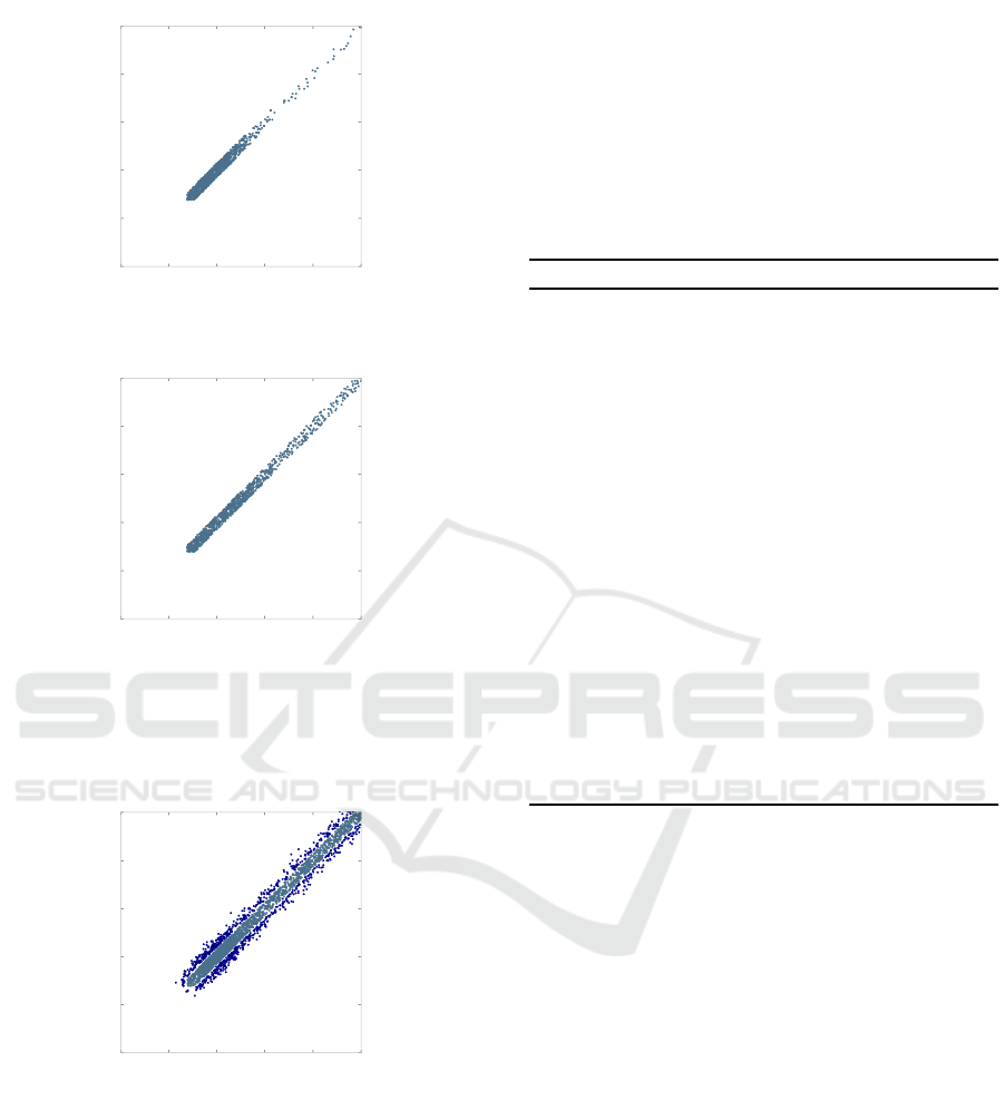
4.1 Selection of Feasible Examples
Selection of feasible examples leads to more homoge-
neously distributed feasible examples as in the origi-
nal distribution of the low-dimensional data subsets,
see Fig. 2. Here the selection of feasible examples in-
creases the point density in the upper right corner and
decreases the point density in the lower left corner,
see Fig. 2(b) in comparison to the original distribution
shown in Fig. 2(a). We propose a sampling Algorithm
1, based on a minimal distance δ of feasible examples
to their nearest feasible neighbors.
Algorithm 1: Selection of feasible examples.
Require: 2-dimensional data set X with n feasi-
ble examples
1: choose t start examples S from X
2: repeat
3: choose t new examples E from X
4: calculate euclidean distance δ of E to
their nearest neighbors in S
5: if δ ≥ ε then
6: append respective examples to S
7: end if
8: until all n examples are processed
9: shuffle S
Figure 1: Pseudocode for the selection of feasible examples.
The minimal distance ε between feasible nearest neighbors
depends on the data set.
The distribution of the feasible examples can dif-
fer a little in homogeneity and shape among the
2-dimensional data subset despite previous scaling.
Therefore the parameters of the procedure have to be
adapted carefully, especially the minimum distance ε
of new examples (E) to the nearest selected neighbors
(S). Preferably, ε is selected in such a way, that the
selection of feasible examples yields round about the
number of examples required for training and valida-
tion. Such ε values yielded in pre-tests good classifi-
cation results, because the resampled data sets main-
tain the integrity of the original data subsets best for
the desired number of training and validation exam-
ples.
4.2 Sampling of Infeasible Examples
Near the Class Boundaries
The sampling procedure of artificial infeasible 2-
dimensional examples near the class boundaries,
see Fig. 3, requires more or less homogeneously dis-
tributed feasible 2-dimensional examples that repre-
sent the whole feasible region.
ICAART 2016 - 8th International Conference on Agents and Artificial Intelligence
98

0.0 0.2 0.4 0.6 0.8 1.0
95th dimension
0.0
0.2
0.4
0.6
0.8
1.0
96th dimension
(a) Initial distribution
0.0 0.2 0.4 0.6 0.8 1.0
95th dimension
0.0
0.2
0.4
0.6
0.8
1.0
96th dimension
(b) Resampled features
Figure 2: 1000 examples of the 95th and 96th dimensions
of the feasible class of the µCHP data set (initial and resam-
pled).
0.0 0.2 0.4 0.6 0.8 1.0
1st dimension
0.0
0.2
0.4
0.6
0.8
1.0
2nd dimension
Figure 3: Resampled examples of the 1st and 2nd dimen-
sion of the feasible class of the µCHP data set with artifi-
cial infeasible examples. The feasible class shown as gray
points is surrounded by artificial infeasible examples (blue
points).
The better the distribution of the feasible exam-
ples, the better will be the distribution of the arti-
ficially generated infeasible examples. But if the
projection of the high-dimensional data set to the 2-
dimensional data sets exhibits a projection error, like
e.g., a hypersphere data set, see (Neugebauer et al.,
2015), then the artificial infeasible examples are not
located near the true class boundary, but near the de-
cision boundary learned by the cascade classifier. We
propose to sample low-dimensional artificial infeasi-
ble examples by disturbing 2-dimensional feasible ex-
amples and identifying new infeasible instances (Γ)
with the help of a certain minimal distance (δ
b
) to
their nearest feasible neighbors, see Algorithm 2.
Algorithm 2: Sampling of infeasible examples.
Require: 2-dimensional data set X with n feasi-
ble examples, where the distance between
infeasibles and their feasible nearest neigh-
bors is ≤ ε
b
in about 95% of cases
1: Y = X + N (µ,σ)) · α
2: calculate euclidean distance δ
b
of all exam-
ples in Y to their nearest neighbors in X
3: if δ
b
≥ ε
b
then
4: examples are infeasible examples (Γ)
5: end if
6: repeat
7: Y = Γ + N (µ,σ) · α
8: calculate euclidean distance δ
b
of all
examples in Y to their nearest neighbors
in X
9: if δ
b
≥ ε
b
then
10: append example to Γ
11: end if
12: until number of examples in Γ is sufficient
13: shuffle Γ
Figure 4: Pseudocode for sampling of artificial infeasible
examples in 2-dimensional space. The factor α for the
standard normal distribution N (µ,σ) and the minimal dis-
tance between feasible examples and their nearest infeasible
neighbors ε
b
depend on the data set.
This procedure turned out to be parameter-
sensitive. The minimal distance between feasible and
infeasible examples ε
b
has to be larger than the mini-
mal distance ε between the selected feasible examples
and preferably also larger than the longest distance
between feasible nearest neighbors. The closer the
infeasible examples are located to the class boundary,
the greater is the improvement of classification speci-
ficity. But the closer the infeasible examples are lo-
cated to the class boundary, the higher is the probabil-
ity, that these artificial infeasible examples could be
located in the region of the feasible class. This phe-
nomenon can hamper classification improvement by
artificial infeasible examples. Therefore a very care-
ful parametrization of the algorithm is necessary.
Improving Cascade Classifier Precision by Instance Selection and Outlier Generation
99

5 EXPERIMENTAL STUDY
In this section, the effect of the proposed data pre-
processing methods on the performance of the cas-
cade classification approach is evaluated on two data
sets. The first data set is an energy time series data set
micro combined heat and power plant (µCHP) power
production time series. The second data set is an ar-
tificial complex data set where the small interesting
class has a Hyperbanana shape. Banana and Hyper-
banana data sets are often used to test new classifiers,
because they are considered as difficult classification
tasks. Therefore we take the test with the Hyper-
banana data set as a meaningful result.
The experimental study is done with cascade clas-
sifiers on each data set. Altogether three classification
experiments are conducted on both data sets. The first
experiment is done without preprocessing (no pre-
pro.), the second with selected feasible examples (fs)
and the third with selected feasibles and artificial in-
feasible examples (fs + infs). For all experiments a
one-class baseline classifier is used. The third experi-
ment is also done with binary baseline classifiers.
The experimental study is divided into a descrip-
tion of the data sets, the experimental setup and the
results.
5.1 Data Sets
The experiments are conducted with simulated µCHP
power output time series and an artificial Hyper-
banana data set. Both data sets have 96 dimensions
(time steps, resp. features).
5.1.1 µCHP
A µCHP is a small decentralized power and heat gen-
eration unit. The µCHP power production time series
are simulated with a µCHP simulation model
1
. The
µCHP simulation model includes a µCHP model, a
thermal buffer and the thermal demand of a building.
A µCHP can be operated in different modes, where
its technical constraints, the constraints of the ther-
mal buffer and the conditions of the thermal demand
of the building are complied. Power output time se-
ries can be either feasible or infeasible depending on
these constraints. The µCHP simulation model calcu-
lates the power production time series for feasible op-
eration modes, but also infeasible power output time
series can be generated, where at least one constraint
is violated. Due to the different constraints the class
1
Data are available for download on
our department website http://www.uni-
oldenburg.de/informatik/ui/forschung/themen/cascade/.
of feasible power production time series consists of
several clusters. For convenience only such feasible
power output time series are chosen, where the power
production is greater than 0 at each time step. Infea-
sible power output time series are sampled from the
whole volume of the infeasible class. In data space
the class of infeasible power output time series occu-
pies a much larger volume than the class of feasible
ones, (Bremer et al., 2010). The classes are severely
imbalanced, but the experiments are conducted with
equal numbers of examples from both classes.
The feasible and infeasible µCHP power output
time series are scaled according to the maximal elec-
trical power production to values between 0 and 1.
5.1.2 Hyperbanana
As far as there is now 96-dimensional Hyperbanana
data set, we have generated a data set from the ex-
tended d-dimensional Rosenbrock function, (Shang
and Qiu, 2006).
f (x) =
d−1
∑
i=1
[100(x
2
i
− x
i+1
)
2
+ (x
i
− 1)
2
] (3)
The small and interesting class, or here also called
feasible class is sampled from the Rosenbrock val-
ley with f (x) < 100 and the infeasible class with
f (x) >= 100 is sampled only near the class bound-
ary to test the sensitivity of the decision boundaries of
the classifiers.
Sampling of the banana shaped valley is done
by disturbing the minimum of the extended 96-
dimensional Rosenbrock function with normally dis-
tributed values (N (0, 1) · β with β ∈ {40,50,60,70}).
The minima of the Rosenbrock function are presented
in (Shang and Qiu, 2006) for different dimensionali-
ties, but the minimum for 96 dimensions is missing.
Therefore we approximated the minimum with regard
to the other minima with −0.99 for the first dimen-
sion and 0.99 for all other dimensions. The procedure
of disturbing and selecting values from the Rosen-
brock valley is repeated with the sampled values until
enough data points are found. As far as it is difficult
to sample the banana “arms” all at the same time, we
sampled them separately by generating points that are
< or > than a certain value and continued sampling
by repeating disturbance and selection with these val-
ues.
Values from all these repetitions were ag-
gregated to one data set and shuffled. Finally
all dimensions (features) x
i
of the data set are
scaled to values between 0 and 1 by x
i
= [x
i
+
(min(x
i
)+offset)]/[max(x
i
)+offset−min(x
i
)+offset]
with offset = 0.2.
ICAART 2016 - 8th International Conference on Agents and Artificial Intelligence
100

The samples generated by this procedure are not
homogeneously distributed in the Rosenbrock valley
and they do not represent all Hyperbanana “arms”
equally.
The 96-dimensional infeasible examples near the
class boundary are sampled in the same way as the
feasible ones but starting with the feasible Hyper-
banana samples and with 100 ≤ f (x) ≤ 500.
5.2 Experimental Setting
The experimental setting is divided into two parts:
data preprocessing and classification. All calculations
are done in Python. The first part, data preprocess-
ing (selection of feasible examples and generation of
infeasible examples) is done according to Sect. 4.1
and Sect. 4.2.
Selection of feasible examples is parametrized dif-
ferently for both data sets as a result of pre-studies.
The pre-studies were conducted with different min-
imal distances ε and ε
b
and evaluated according to
the number of resulting examples and their distribu-
tion in the 2-dimensional data subset. For the µCHP
data set instance selection is parametrized as follows,
the minimal distance between feasible examples is
set to ε = 0.001 and the number of new examples
used for each iteration t is set to t = 1000. Gener-
ation of artificial infeasible examples is parameter-
ized with n = 15000 initially feasible examples distur-
bance = N (0, 0.01) · α with α = 1 and minimal dis-
tance between infeasible examples and their nearest
feasible neighbors ε
b
= 0.025. For the Hyperbanana
data set the instance selection parameters are set to
ε = 0.002 and t = 1000 and parameters for generating
artificial infeasible examples are set to n = 20000, dis-
turbance = N (0,0.02) · α with α = 1 and ε
b
= 0.002.
The second part of the experimental study, the
three classification experiments, are done with the
cascade classifier, see Sect. 3, with different base-
line classifiers from SCIKIT-LEARN, (Pedregosa et al.,
2011), a One-Class SVM (OCSVM) and two binary
classifiers, k-nearest neighbors (kNN) and Support
Vector Machines (SVMs). The OCSVM baseline
classifier is used for all three experiments. The two
binary classifiers kNN and binary SVM are used for
the third experiment with both preprocessing methods
(fs + infs).
All experiments are conducted identically on both
data sets except for the parametrization. For all exper-
iments the number of feasible training examples N is
varied in the range of N = {1000, 2000, . . . , 5000} for
the µCHP data set and N = {1000,2000,...,10000}
for the Hyperbanana data set. For binary classifica-
tion N infeasible examples are added to the N feasible
training examples.
Parameter optimization is done with grid-search
on separate validation sets with the same number of
feasible examples N as the training sets and also N
artificial infeasible examples for the third experiment.
For the first experiment (no prepro.) and the second
experiment (fs) the parameters are optimized accord-
ing to true positive rates (TP rate or only TP), (TP rate
= (true positives) / (number of feasible examples)).
For the third experiment, where the validation
is done with N additional infeasible examples, pa-
rameters are optimized according to accuracy (acc
= (true positives + true negatives)/(number of posi-
tive examples + number of negative examples)). The
OCSVM parameters are optimized in the ranges ν ∈
{0.0001,0.0005,0.001, 0.002, . . . , 0.009, 0.01}, γ ∈
{50,60,...,200}, the SVM parameters in C ∈
{1,10,50,100,500,1000,2000}, γ ∈ {1,5,10,15,20}
and the kNN parameter in k ∈ {1,2,...,26}.
Evaluation of the trained classifiers is done on
a separate independent data set with 10000 feasible
and 10000 real infeasible 96-dimensional examples
according to TP and TN rates for varying numbers
of training examples N. The classification results
could be evaluated with more advanced measures, see
e.g. (He and Garcia, 2009; Japkowicz, 2013). For bet-
ter comparability of the results on both data sets and
the option to distinguish effects on the classification
of feasible and infeasible examples we use the simple
TP and TN rates. TN rates on both data sets are dif-
ficult to compare, because the infeasible µCHP power
output time series are distributed in the whole region
of infeasible examples, while the infeasible Hyper-
banana examples are distributed only near the class
boundary. As far as most classification errors occur
near the class boundary, the TN rates of the Hyper-
banana set are expected to be lower than the TN rates
on the µCHP data set.
5.3 Results
The proposed data preprocessing methods, selection
of feasible examples and generation of artificial in-
feasible examples show an increase in classification
performance of the cascade classifier in the experi-
ments.
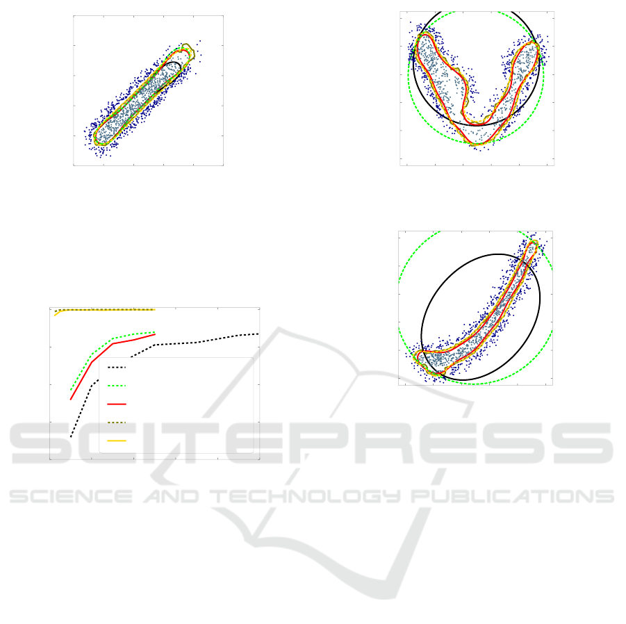
On both data sets (µCHP and Hyperbanana) data
preprocessing leads to more precise decision bound-
aries than without data preprocessing, see Fig. 5
and Fig. 7. This can be also seen in the TP and TN
rates of the classification results, see Fig. 6 and Fig. 8.
For the µCHP data set, all three experiments lead
to TN rates of 1, therefore only the TP rates are plot-
ted in Fig. 6. But high TN rates for the µCHP data set
Improving Cascade Classifier Precision by Instance Selection and Outlier Generation
101

0.2 0.3 0.4 0.5 0.6 0.7
1st dimension
0.2
0.3
0.4
0.5
0.6
0.7
2nd dimension
Figure 5: Decision boundaries on the 1st and 2nd dimension
of the µCHP trained with N = 1000 feasible (+ N = 1000
infeasible) training examples, no prepro. (dashed black),
fs (dashed green), OCSVM(fs + infs) (red), kNN(fs + infs)
(olive) and SVM(fs + infs) (yellow). The gray points indi-
cate 500 of the selected feasible training examples and the
blue points 500 of the artificial infeasible examples.
0 2000 4000 6000 8000 10000
N
0.6
0.7
0.8
0.9
1.0
TP
OCSVM (no prepro.)
OCSVM (fs)
OCSVM (fs + infs)
kNN (fs + infs)
SVM (fs + infs)
Figure 6: TP rates on the µCHP data set for different pre-
processing steps and different baseline classifiers.
do not necessarily mean, that further infeasible time
series are classified correctly. The applied infeasible
test examples are taken from the whole volume of the
large infeasible class and therefore most of the ex-
amples are not located near the class boundary. The
first experiment without data preprocessing (no pre-
pro.) yields the lowest TP rates of all experiments
for all numbers of training values N and the second
experiment with selection of feasible examples (fs)
leads already to higher TP rates. The third experi-
ment with selection of feasible examples and artifi-
cial infeasible examples (fs + infs) leads to different
results with the OCSVM baseline classifier and the
binary SVM and kNN baseline classifiers. While the
OCSVM(fs + infs) achieves slightly lower TP rates
than OCSVM(fs) in the second experiment, the bi-
nary baseline classifiers SVM(fs + infs) and kNN(fs
+ infs) achieve TP rates near 1.
For the Hyperbanana data set with a more com-
plex data structure, data preprocessing influences the
TP rates, see Fig. 8(a) and the TN rates, Fig. 8(b) of
the classification results. In the first experiment (no
0.0 0.2 0.4 0.6 0.8 1.0
1st dimension
0.0
0.2
0.4
0.6
0.8
1.0
2nd dimension
(a) 2d-boundaries on dim. 1/2
0.0 0.2 0.4 0.6 0.8 1.0
95th dimension
0.0
0.2
0.4
0.6
0.8
1.0
96th dimension
(b) 2d-boundaries on dim. 95/96
Figure 7: Decision boundaries on the Hyperbanana data
set trained with N = 1000 feasible (+ N = 1000 infeasible)
training examples, no prepro. (dashed black), fs (dashed
green), OCSVM(fs + infs) (red), kNN(fs + infs) (olive) and
SVM(fs + infs) (yellow). The gray points indicate 500 of
the selected feasible training examples and the blue points
500 of the artificial infeasible examples.
prepro.) and second experiment (fs) the classifica-
tion achieves relatively high TP rates and at the same
time the lowest TN rates of all experiments due to
too large decision boundaries, see Fig. 7. The third
experiment (fs + infs) revealed an opposed behav-
ior of the OCSVM baseline classifier and the SVM
and kNN baseline classifiers. The OCSVM(fs + infs)
achieves lower TP rates than the OCSVM in the pre-
vious experiments but also the highest TN rates of all
experiments. SVM and kNN baseline classifiers with
(fs + infs) achieve the highest TP rates of all experi-
ments and at the same time lower TN rates than the
OCSVM(fs + infs).
In summary, data preprocessing increases the clas-
sification performance of the cascade classifier on
both data sets. While the selection of feasible ex-
amples increases the classification performance, arti-
ficial infeasible examples can lead to an even greater
increase depending on the data set and the baseline
classifier.
ICAART 2016 - 8th International Conference on Agents and Artificial Intelligence
102

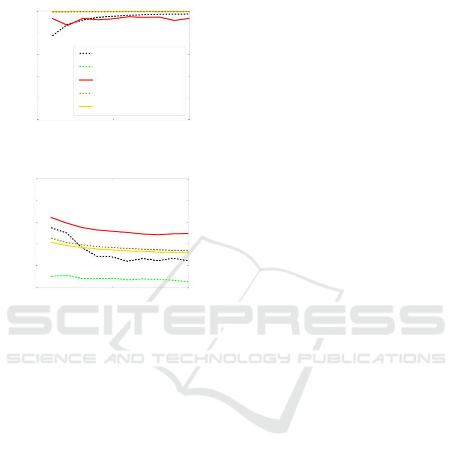
0 5000 10000
N
0.0
0.2
0.4
0.6
0.8
1.0
TP
OCSVM (no prepro.)
OCSVM (fs)
OCSVM (fs + infs)
kNN (fs + infs)
SVM (fs + infs)
(a) TP rates on a differently preprocessed Hyperbanana
set
0 5000 10000
N
0.0
0.2
0.4
0.6
0.8
1.0
TN
(b) TN rates on a differently preprocessed Hyper-
banana set
Figure 8: TP and TN rates on the Hyperbanana data set for
different preprocessing steps and different baseline classi-
fiers. The legend in Fig. 8(a) is also valid for Fig. 8(b). The
green line of OCSVM(fs) in Fig. 8(a) is covered by the olive
and the yellow lines.
6 CONCLUSIONS
In this paper, we proposed two data preprocessing
methods to improve the performance of the cascade
classification model (selection of feasible examples
and generation of artificial infeasible examples). In
the experimental study, we showed for a µCHP power
output time series data set and an artificial and com-
plex Hyperbanana data set, that data preprocessing
increases the performance of the cascade classifier.
Selection of feasible examples leads to more repre-
sentative training data and artificial infeasible exam-
ples lead to more precise decision boundaries of the
low-dimensional classifiers. Depending on the data
set and the baseline classifier, the application of both
data preprocessing methods yields the best classifica-
tion performance. The application of only one data
preprocessing method (selection of feasible exam-
ples) and no data preprocessing yielded always worse
results, lower TP rates on the µCHP data set and es-
pecially very low TN rates on the Hyperbanana data
set.
In summary, the proposed data preprocessing
methods for the cascade classifier are very sensitive
concerning the parametrization, but a careful parame-
ter choice increases the classification performance.
We plan to generalize our cascade classification
model in future work in such a way, that it can deal
with data sets with more complex data structures, e.g.,
the small and interesting class consists of several clus-
ters or the low-dimensional data subsets employ a
data structure that can not be learned easily like a
butterfly-like shape.
Furthermore, we intend to evaluate the proposed
data preprocessing methods on such data sets.
ACKNOWLEDGEMENT
This work was funded by the Ministry for Science and
Culture of Lower Saxony with the PhD program Sys-
tem Integration of Renewable Energy (SEE).
REFERENCES
Bagnall, A., Davis, L. M., Hills, J., and Lines, J. (2012).
Transformation based ensembles for time series clas-
sification. In Proceedings of the Twelfth SIAM Inter-
national Conference on Data Mining, Anaheim, Cali-
fornia, USA, April 26-28, 2012., pages 307–318.
B
´
anhalmi, A., Kocsor, A., and Busa-Fekete, R. (2007).
Counter-example generation-based one-class classifi-
cation. In Kok, J. N., Koronacki, J., Mantaras, R. L.,
Matwin, S., Mladeni
˜
c, D., and Skowron, A., editors,
Machine Learning: ECML 2007, volume 4701 of
Lecture Notes in Computer Science, pages 543–550.
Springer Berlin Heidelberg.
Bellinger, C., Sharma, S., and Japkowicz, N. (2012). One-
class versus binary classification: Which and when?
In Machine Learning and Applications: ICMLA, 2012
11th International Conference on, volume 2, pages
102–106.
Blachnik, M. (2014). Ensembles of instance selection meth-
ods based on feature subset. Procedia Computer
Science, 35(0):388 – 396. Knowledge-Based and
Intelligent Information &amp; Engineering Systems
18th Annual Conference, KES-2014 Gdynia, Poland,
September 2014 Proceedings.
Bremer, J., Rapp, B., and Sonnenschein, M. (2010). Sup-
port vector based encoding of distributed energy re-
sources’ feasible load spaces. In Innovative Smart
Grid Technologies Conference Europe IEEE PES.
Garcia, S., Derrac, J., Cano, J., and Herrera, F. (2012).
Prototype selection for nearest neighbor classifica-
tion: Taxonomy and empirical study. IEEE Transac-
Improving Cascade Classifier Precision by Instance Selection and Outlier Generation
103

tions on Pattern Analysis and Machine Intelligence,
34(3):417–435.
He, H. and Garcia, E. (2009). Learning from imbalanced
data. Knowledge and Data Engineering, IEEE Trans-
actions on, 21(9):1263–1284.
Jankowski, N. and Grochowski, M. (2004). Comparison
of instances seletion algorithms i. algorithms survey.
In Rutkowski, L., Siekmann, J., Tadeusiewicz, R.,
and Zadeh, L., editors, Artificial Intelligence and Soft
Computing - ICAISC 2004, volume 3070 of Lecture
Notes in Computer Science, pages 598–603. Springer
Berlin Heidelberg.
Japkowicz, N. (2013). Assessment Metrics for Imbalanced
Learning, pages 187–206. John Wiley & Sons, Inc.
Lin, W.-J. and Chen, J. J. (2013). Class-imbalanced classi-
fiers for high-dimensional data. Briefings in Bioinfor-
matics, 14(1):13–26.
Liu, H., Motoda, H., Gu, B., Hu, F., Reeves, C. R., and
Bush, D. R. (2001). Instance Selection and Construc-
tion for Data Mining, volume 608 of The Springer In-
ternational Series in Engineering and Computer Sci-
ence. Springer US, 1 edition.
Neugebauer, J., Kramer, O., and Sonnenschein, M. (2015).
Classification cascades of overlapping feature ensem-
bles for energy time series data. In Woon, W. L.,
Aung, Z., and Madnick, S., editors, Data Analytics
for Renewable Energy Integration. Springer. in print.
Pedregosa, F., Varoquaux, G., Gramfort, A., Michel, V.,
Thirion, B., Grisel, O., Blondel, M., Prettenhofer,
P., Weiss, R., Dubourg, V., Vanderplas, J., Passos,
A., Cournapeau, D., Brucher, M., Perrot, M., and
Duchesnay, E. (2011). Scikit-learn: Machine learning
in Python. Journal of Machine Learning Research,
12:2825–2830.
Shang, Y.-W. and Qiu, Y.-H. (2006). A note on the extended
rosenbrock function. Evol. Comput., 14(1):119–126.
Tax, D. M. J. and Duin, R. P. W. (2002). Uniform ob-
ject generation for optimizing one-class classifiers. J.
Mach. Learn. Res., 2:155–173.
Toma
ˇ
sev, N., Buza, K., Marussy, K., and Kis, P. B. (2015).
Hubness-aware classification, instance selection and
feature construction: Survey and extensions to time-
series. In Sta
´
nczyk, U. and Jain, L. C., editors, Feature
Selection for Data and Pattern Recognition, volume
584 of Studies in Computational Intelligence, pages
231–262. Springer Berlin Heidelberg.
Tsai, C.-F., Eberle, W., and Chu, C.-Y. (2013). Ge-
netic algorithms in feature and instance selection.
Knowledge-Based Systems, 39(0):240–247.
Wilson, D. and Martinez, T. (2000). Reduction tech-
niques for instance-based learning algorithms. Ma-
chine Learning, 38(3):257–286.
Zhuang, L. and Dai, H. (2006). Parameter optimization
of kernel-based one-class classifier on imbalance text
learning. In Yang, Q. and Webb, G., editors, PRICAI
2006: Trends in Artificial Intelligence, volume 4099
of Lecture Notes in Computer Science, pages 434–
443. Springer Berlin Heidelberg.
ICAART 2016 - 8th International Conference on Agents and Artificial Intelligence
104