On the Decomposition of Min-based Possibilistic Inﬂuence Diagrams

Salem Benferhat

, Hadja Faiza Khellaf-Haned

and Ismahane Zeddigha

CRIL, Universit

e d’Artois, Rue Jean Souvraz, SP 18 62307, Lens Cedex, France

RIIMA, Universit

e des Sciences et de la Technologie Houari Boumediene, BP 32 El Alia Bab Ezzouar, Alger, Alg

erie

Keywords:

Decision Theory, Possibility Theory, Possibilistic Networks, Possibilistic Inﬂuence Diagrams.

Abstract:

Min-based possibilistic inﬂuence diagrams allow a compact modelling of decision problems under uncertainty.

Uncertainty and preferential relations are expressed on the same structure by using ordinal data. Like proba-

bilistic inﬂuence diagrams, min-based possibilistic inﬂuence diagrams contain three types of nodes: chance,

decision and utility nodes. Uncertainty is described by means of possibility distributions on chance nodes and

preferences are expressed as satisfaction degrees on utility nodes.

In many applications, it may be natural to represent expert knowledge and preferences separately and treat all

nodes similarly. This paper shows how an inﬂuence diagram can be equivalently represented by two possibilis-

tic networks: the ﬁrst one represents knowledge of an agent and the second one represents agent’s preferences.

Thus, the decision evaluation process is based on more compact possibilistic network.

1 INTRODUCTION

Decision making under uncertainty (Whalen, 1984),

(Denardo et al., 2012), (Anzilli, 2013), (Dubois et al.,

2013) plays an important role in Artiﬁcial Intelligence

(AI) applications. Several decision making tools have

been developed to assist decision makers in their

tasks: simulation techniques, dynamic programming

(Sniedovich, 2010), logical decision models (Dubois

et al., 1998) and graphical decision models (Zhang,

2013), (Garcia and Sabbadin, 2006). Using graphical

models, authors in (Boutouhami and Khellaf, 2015)

have proposed an approximate approach for comput-

ing optimal qualitative possibilistic optimistic deci-

sion in the context of optimistic criteria. They showed

that it comes down to computing a normalization de-

gree of the moral graph associated to the resulting

graph obtained by merging preferences and knowl-

edge represented by two min-based possibilistic net-

works.

This paper also focuses on graphical decision

models which provide efﬁcient decision tools by al-

lowing a compact representation of decision prob-

lems under uncertainty (Shenoy, 1994). Most of de-

cision graphical models are based on Inﬂuence Dia-

grams (ID) (Howard and Matheson, 1984), (Zhang,

1998) for representing decision maker’s beliefs and

preferences on sequences of decisions to be made

under uncertainty. The evaluation of Inﬂuence Di-

agrams ensures optimal decisions while maximizing

the decision maker’s expected utilities (Tatman and

Shachter, 1990), (Zhang, 1998), (Dubois and Prade,

1988). Min-based (or qualitative) possibilistic Inﬂu-

ence Diagrams ”PID” (Garcia and Sabbadin, 2006)

allow a gradual expression of both agent’s prefer-

ences and knowledge. The graphical part of possi-

bilistic Inﬂuence Diagrams is exactly the same as the

one of standard Inﬂuence Diagrams. Uncertainty is

expressed by possibility degrees and preferences are

considered as satisfaction degrees.

Unlike probabilistic decision theory which is

based on one expected utility criteria to evaluate opti-

mal decisions, a qualitative possibilistic decision the-

ory (Dubois et al., 1999), (Dubois et al., 2001) of-

fers several qualitative utility criteria for decision ap-

proaches under uncertainty. Among these criteria,

one can mention the pessimistic and optimistic utili-

ties proposed in (Dubois and Prade, 1995), the binary

utility proposed in (Giang and Shenoy, 2005), etc.

As standard Inﬂuence Diagrams, direct (Garcia and

Sabbadin, 2006) and an indirect methods (Garcia and

Sabbadin, 2006), (Guezguez et al., 2009) have been

proposed to evaluate a min-based PID. Besides, Inﬂu-

ence Diagrams represent agent’s beliefs and prefer-

ences on the same structure and they operate on three

types of nodes: chance, decision and utility nodes.

In practice, it will be easier for an agent to express

its knowledge and preferences separately. Further-

Benferhat, S., Khellaf-Haned, H. and Zeddigha, I.

On the Decomposition of Min-based Possibilistic Inﬂuence Diagrams.

DOI: 10.5220/0005703501170128

In Proceedings of the 8th International Conference on Agents and Artiﬁcial Intelligence (ICAART 2016) - Volume 2, pages 117-128

ISBN: 978-989-758-172-4

117

more, it is more simple to treat all nodes in the same

way. In (Benferhat et al., 2013), authors have pro-

posed a new compact graphical model for represent-

ing decision making under uncertainty based on the

use of possibilistic networks. Agent’s knowledge and

preferences are expressed in qualitative way by two

distinct qualitative possibilistic networks. This new

representation, for decision making under uncertainty

based on min-based possibilistic networks, beneﬁts

from the simplicity of possibilistic networks.

In this paper, we show how to decompose an ini-

tial min-based Inﬂuence Diagram into two min-based

possibilistic networks: the ﬁrst one represents agent’s

beliefs and the second one encodes its preferences.

Then, we deﬁne the required steps for splitting a qual-

itative Inﬂuence Diagram into two min-based possi-

bilistic networks preserving the same possibility dis-

tribution and the same qualitative utility. This proce-

dure allows us to obtain a more compact (in terms

of dependence) qualitative possibilistic network for

computing optimal decisions. This decomposition

process provides also the opportunity to exploit the in-

ference algorithms (Ajroud et al., 2012), (Amor et al.,

2003) developed for min-based possibilistic networks

to solve qualitative Inﬂuence Diagrams.

The rest of this paper is organized as follows:

next section brieﬂy recalls basic concepts of possibil-

ity theory, min-based possibilistic networks and min-

based PID. Section 3 describes how the decompo-

sition process can be efﬁciently used for encoding

an Inﬂuence Diagram into two possibilistic networks.

Section 4 gives related works. Section 5 concludes

the paper.

2 BACKGROUND

2.1 Basic Concepts of Possibility Theory

This section gives a brief refresher on possibility the-

ory (Dubois and Prade, 1988) which is issued from

fuzzy sets theory (Zadeh, 1978).

Let X = {X

, ..., X

} be a set of variables. We de-

note by D

= {x

, ..., x

} the domain associated with

the variable X

. x

i j

denotes the jth instance of X

. The

universe of discourse is denoted by Ω = ×

∈V

which is the Cartesian product of all variables domain

in X . Each element ω ∈ Ω is called an interpretation

which represents a possible state of Ω. It is denoted

by ω = (x

, ..., x

N j

). φ, ψ... represent events, namely

subsets of Ω.

A basic element in a possibility theory is the no-

tion of possibility distribution π which corresponds to

a mapping from Ω to the scale [0, 1]. This distribution

encodes available knowledge on real world. π(ω) = 1

means that ω is completely possible and π(ω) = 0

means that it is impossible for ω to represent the real

world. A possibilistic scale can be interpreted in or-

dinal or numerical way. A possibility distribution π is

said to be normalized, if max

π(ω) = 1.

Given a possibility distribution π on the universe

discourse Ω, two dual measures are deﬁned for each

event φ ⊆ Ω: Possibility measure Π(φ) and Neces-

sity measure N(φ). The ﬁrst one evaluates to what

extent φ is consistent with our knowledge encoded

by π, namely Π(φ) = max

ω∈Ω

{π(ω) : ω |= φ}. The sec-

ond one, evaluates at which level φ is certainly im-

plied by our knowledge represented by π, namely

N(φ) = 1 − Π(¬φ).

The possibilistic conditioning consists in the revi-

sion of our initial knowledge, encoded by a possibility

distribution π by the arrival of a new certain informa-

tion φ ⊆ Ω. The initial distribution π is then replaced

by another one, denoted π

= π(. | φ). The two inter-

pretations relative to the possibilistic scale (qualita-

tive and quantitative) induce two deﬁnitions of possi-

bilistic conditioning (Amor et al., 2002), (Bouchon-

Meunier et al., 2002): product-based conditioning

and min-based conditioning. In this paper, we use the

last one deﬁned by:

π(ω |

min

φ) =







1 If π(ω) = Π(φ) and ω |= φ

π(ω) If π(ω) < Π(φ) and ω |= φ

0 oterhwise

(1)

Similarly, possibility theory offers several deﬁni-

tions of independence relation (Amor et al., 2002),

(de Campos and Huete, 1999). As we interpret the un-

certainty scale in ordinal manner, we will used the so-

called min-based independence relation, initially de-

ﬁned as a non-interactivity relation by Zadeh (Zadeh,

1978). This relation is obtained by using the min-

based conditioning (Equation 1) and it is deﬁned by:

∀x, y, z Π(x ∧ y | z) = min(Π(x | z), Π(y | z)). (2)

2.2 Min-based Possibilistic Networks

In a possibility theory framework, there are two ways

to deﬁne possibilistic networks according to the possi-

bilistic conditioning. In this paper, we only focus on

min-based possibilistic networks. A min-based pos-

sibilistic network (Borgelt et al., 1998) over a set of

variables X denoted by ΠG

min

= (G, π) is character-

ized by:

1. A Graphical Component: which is represented

by a Directed Acyclic Graph (DAG) where nodes

correspond to variables and arcs represent depen-

dence relations between variables.

ICAART 2016 - 8th International Conference on Agents and Artiﬁcial Intelligence

118

2. Numerical Components: these components

quantify different links in the DAG by using lo-

cal possibility distributions for each node X in the

context of its parents denoted by Par(X). More

precisely:

• For every root node X (Par(X) =

0), uncer-

tainty is represented by a priori possibility de-

gree π(x) for each instance x ∈ D

, such that

max

x∈Ω

π(x) = 1.

• For the rest of the nodes (Par(X ) 6=

0), uncer-

tainty is represented by the conditional possi-

bility degree π(x | u

) for each instance x ∈

and for any instance u

∈ D

Par(X)

(where

Par(X)

represents the Cartesian product of

all variables domain in Par(X)), such that

max

x∈Ω

π(x | u

) = 1, for any u

The set of a priori and conditional possibility degrees

induces a unique joint possibility distribution π

de-

ﬁned by:

, ..., X

) = min

i=1..N

π(X

| U

). (3)

The most common task performed on possibilistic

networks is the possibilistic inference which consists

in determining how the realization of speciﬁc values

of some variables called (observations or evidence)

affects the remaining variables (Huang and Darwiche,

1996).

2.3 Min-based Possibilistic Inﬂuence

Diagrams

Like standard Inﬂuence Diagrams (Lauritzen and

Nilsson, 2001)(Zhang, 2013), PID

have two compo-

nents: the graphical part which is exactly the same

as the one of standard Inﬂuence Diagrams and the

numerical part which consists in evaluating different

links in the graph. The uncertainty is expressed by

possibility degrees and preferences are considered as

satisfaction degrees.

In a min-based possibilistic Inﬂuence Dia-

gram (qualitative possibilistic ID), denoted by

ΠID

min

, π

min

, µ

min

), both agent’s knowledge and

preferences are expressed in a qualitative setting. This

is achieved by ordering the different states of the

world and providing a preference relation between

different consequences.

1. A Graphical Component: which is represented

by a DAG, denoted by G

= (X , A) where X =

C ∪ D ∪U represents a set of variables containing

three different kinds of nodes: chance, decision

and utility nodes. A is a set of arcs representing

either causal inﬂuences or information inﬂuences

between variables.

• Chance Nodes: are represented by cir-

cles. They represent state variables X

∈ C =

, ..., X

}. Chance nodes reﬂect uncertain

factors of a decision problem. A combination

x = {x

, ..., x

n j

} of state variable values repre-

sents a state.

• Decision Nodes: are represented by rectangles.

They represent decision variables D

∈ D =

, ..., D

} which depict decision options. A

combination d = {d

, ..., d

p j

} of values repre-

sents a decision.

• Utility Nodes: or value nodes V

∈ V =

, ...,V

} are represented by diamonds. They

represent local utility functions (local satisfac-

tion degrees) µ

∈ {µ

, ..., µ

A conventional assumption that an Inﬂuence Di-

agram must respect is that utility nodes have no

children.

2. Numerical Components: After specifying the

structure of an Inﬂuence Diagram, uncertainty is

described by means of a priori and conditional

possibility distributions relative to chance nodes.

Possibility distributions are deﬁned on the scale

L = [0, 1] and they are assumed to be normalized.

In addition, decision maker should quantify value

nodes, on utility scale U, to express their utilities

(which may not be normalized). These compo-

nents quantify different links in the DAG as fol-

lows:

• For every chance node X ∈ C , uncertainty is

represented by:

– If X is a root node, then a priori possibility

degree π

(x) will be associated for each in-

stance x ∈ D

, such that max

x∈D

(x) = 1.

– If X has parents, the conditional possibil-

ity degree π

(x | u

) will be associated for

each instance x ∈ D

and u

∈ D

Par(X)

∈Par(X)

, such that max

x∈D

(x | u

) = 1,

for any u

• Decision nodes are not quantiﬁed. Indeed, a

value of decision node D

is deterministic, it

will be ﬁxed by the decision maker.

Once a decision d = {d

, ..., d

p j

} ∈ D is ﬁxed,

chance nodes of the min-based Inﬂuence Dia-

gram form a qualitative possibilistic network in-

duces a unique joint conditional possibility dis-

tribution relative to chance node interpretations

x = {x

, ..., x

n j

}, in the context of d.

min

(x | d) = min

i=1..n

| u

). (4)

On the Decomposition of Min-based Possibilistic Inﬂuence Diagrams

119

where x

∈ D

and u

∈ D

Par(X

)

∈Par(X

),D

∈Par(X

)

∪ D

• For each utility node V

k=1..q

∈ V , ordinal val-

ues µ

) are assigned to every possible in-

stantiations u

of the parent variables Par(V

Ordinal values µ

represent satisfaction degrees

associated with local instantiations of parents

variables.

The global satisfaction degree µ

min

(x, d) relative

to the global instantiation (x, d) of all variables

(chance and decision nodes) can be computed as

the minimum of the local satisfaction degrees:

min

(x, d) = min

k=1..q

). (5)

where u

∈ D

Par(V

)

= ×

∈Par(V

),D

∈Par(V

)

∪

A qualitative Inﬂuence Diagram is evaluated in or-

der to identify the optimal strategy δ

∗

, maximizing

one of the possibilistic qualitative utilities. In fact, a

strategy δ assigns an instantiation d to each global in-

stantiation x of the state variables.

3 DECOMPOSITION OF

MIN-BASED POSSIBILISTIC

INFLUENCE DIAGRAM

This section discusses the main contributions of this

paper. Our aim is to show that a qualitative PID

can be modelled by two possibility distributions, one

representing agent’s beliefs and the other represent-

ing the qualitative utility. So, we propose a decom-

position process of min-based possibilistic Inﬂuence

Diagram ΠID

min

, π

min

, µ

min

) into two min-based

possibilistic networks:

1. Agent’s knowledge ΠK

min

= (G

, π). This qual-

itative possibilistic network should codify the

same joint conditional possibility distribution π

min

induced by the PID.

2. Agent’s preferences ΠP

min

= (G

, µ). Again, this

preference-based possibilistic network must cod-

ify the same qualitative utility µ

min

induced by the

PID.

In what follows, the decomposition process of the

Inﬂuence Diagram ΠID

min

, π

min

, µ

min

) into two

qualitative possibilistic networks is presented.

3.1 The Construction of a

Knowledge-based Qualitative

Possibilistic Network

The knowledge-based qualitative possibilistic net-

work ΠK

min

= (G

, π) encodes agent’s beliefs. It in-

duces a unique possibility distribution π

using Equa-

tion 3. The graphical component G

of the new qual-

itative possibilistic network ΠK

min

is deﬁned on the

set of variables Y = X ∪ D = {Y

, ...,Y

n+p

} of chance

and decision nodes (where n = |X | and p = |D|). The

construction of such network is performed in three

steps:

• Each decision node D

will be transformed into

a chance node representing the total ignorance,

namely:

∀D

∈ D, π(d

| u

) = 1. (6)

for each instance d

∈ D

and u

∈ D

Par(D

)

• All state nodes remain unchanged:

∀X

∈ C , π(x

| u

) = π

| u

) (7)

for each instance x

∈ D

and u

∈ D

Par(X

)

• All utility nodes {V

, ...,V

} and their associated

edges are removed.

The building of the knowledge-based possibilistic

network ΠK

min

can be summarized by Algorithm 1.

The new min-based possibilistic network ΠK

min

Data: ΠID

min

, π

min

, µ

min

), a min-based

PID.

Result: ΠK

min

= (G

, π), knowledge-based

network.

begin

foreach D

∈ D do

Transform each decision node D

into

chance node using Equation 6.

end

foreach X

∈ C do

Quantify each chance node X

using

Equation 7.

end

Remove utility nodes {V

, ...,V

end

Algorithm 1: Building knowledge-based network.

, π) induces a unique joint possibility distribution

deﬁned by the min-based chain rule (Equation 3).

The following proposition ensures that the joint pos-

sibility distribution induced by the new possibilistic

network ΠK

min

encodes the same states represented

by the Inﬂuence Diagram ΠID

min

ICAART 2016 - 8th International Conference on Agents and Artiﬁcial Intelligence

120

Proposition 1. Let ΠK

min

= (G

, π) be a min-based

possibilistic network obtained using Algorithm 1. The

joint possibility distribution π

induced by ΠK

min

equal to the one induced by the Inﬂuence Diagram

ΠID

min

. Namely,

, ...,Y

n+p

) = π

min

, ..., X

| D

, ..., D

)

= min

∈C

| U

)

(8)

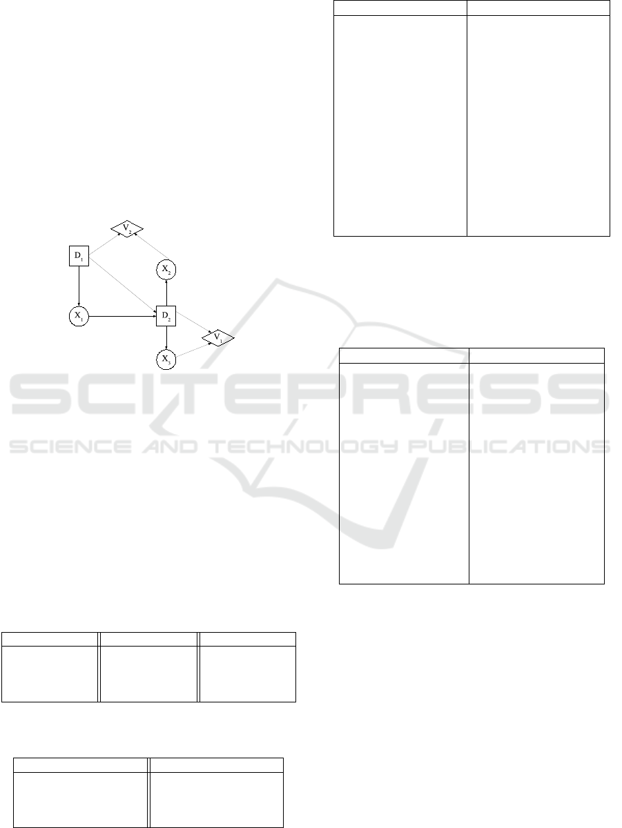
Example 1. Let us consider a simple decision prob-

lem represented by a min-based Inﬂuence Diagram

ΠID

min

, π

min

, µ

min

). The graphical component

is given by Figure 1. It contains three chance

nodes C = {X

, X

}, two decision nodes D =

, D

} and two utility nodes V = {V

}. We sup-

pose that all variables are binary.

Figure 1: An example of inﬂuence diagram.

The numerical components are represented by

conditional possibility distributions associated with

chance nodes X

, X

and qualitative utilities for

the value node V

and V

, in the context of their par-

ents. Indeed, conditional possibilities are represented

in Tables 1. Utilities for V

and V

are represented in

Table 2. It should be noted that utilities for V

is not

normalized.

The joint conditional possibility distribution π

min

induced by the Inﬂuence Diagram ΠID

min

, using

Equation 4, is given by Table 3.

Table 1: Initial possibility distributions π

on X

| D

, X

and X

| D

) X

| D

) X

| D

)

1 x

.3 x

¬d

.4 x

¬d

1 x

¬d

¬x

.2 ¬x

1 ¬x

¬x

¬d

1 ¬x

¬d

.4 ¬x

¬d

Table 2: Initial qualitative utilities µ

on X

, D

and µ

, D

) X

, D

)

.2 x

¬d

.3 x

¬d

¬x

1 ¬x

¬x

¬d

0 ¬x

¬d

Table 3: The joint conditional possibility distribution π

min

on X

, X

given D

, D

min

.3 ¬x

¬d

1 ¬x

¬d

.3 ¬x

¬d

.4 ¬

¬x

¬d

¬x

.3 ¬x

¬x

¬d

.8 ¬x

¬x

¬d

¬x

¬d

.3 ¬x

¬x

¬d

¬x

¬d

.4 ¬x

¬x

¬d

¬x

1 ¬x

¬x

¬d

.3 ¬x

¬x

¬d

¬x

¬d

.4 ¬

¬x

¬d

¬x

¬d

.4 ¬x

¬x

¬d

¬x

.4 ¬x

¬x

¬d

.4 ¬x

¬x

¬d

¬x

¬d

.4 ¬x

¬x

¬d

¬x

¬d

.4 ¬x

¬x

¬d

The global satisfaction degree

min

, D

, X

) generated by the Inﬂu-

ence Diagram ΠID

min

can be computed using

Equation 5. The results are reported in Table 4.

Table 4: Global qualitative utilities µ

min

, D

, X

min

.2 ¬d

¬x

.5 ¬d

¬x

.1 ¬d

¬x

.1 ¬d

¬x

.2 ¬d

¬x

.5 ¬d

¬x

.1 ¬d

¬x

.1 ¬d

¬x

¬d

.3 ¬d

¬d

¬x

0 ¬d

¬d

¬x

¬d

¬x

.1 ¬d

¬d

¬x

¬d

¬x

0 ¬d

¬d

¬x

¬d

¬x

.3 ¬d

¬d

¬x

¬d

¬x

0 ¬d

¬d

¬x

¬d

¬x

.1 ¬d

¬d

¬x

¬d

¬x

0 ¬d

¬d

¬x

We propose to decompose the Inﬂuence Diagram

ΠID

min

given in Figure 1 into two qualitative pos-

sibilistic networks. The ﬁrst min-based possibilistic

network ΠK

min

= (G

, π) describes agent’s knowl-

edge, the second one ΠP

min

= (G

, µ) will express its

preferences.

Let us proceed to build the knowledge-based network

ΠK

min

= (G

, π) using Algorithm 1. The graphical

component G

is given by Figure 2. In fact, the

graphical component G

corresponds to the Inﬂuence

Diagram of Figure 1 from which we removed the util-

ity nodes.

Using Algorithm 1, the initial possibility distribu-

tion associated with ΠK

min

are given by Tables 5, 6

and 7.

On the Decomposition of Min-based Possibilistic Inﬂuence Diagrams

121

Figure 2: Knowledge-based possibilistic network.

Table 5: Initial possibility distribution ΠK

min

on X

| D

and X

| D

π(X

| D

) X

π(X

| D

) X

π(X

| D

)

1 x

.3 x

¬d

.4 x

¬d

1 x

¬d

¬x

.2 ¬x

1 ¬x

¬x

¬d

1 ¬x

¬d

.4 ¬x

¬d

Table 6: Initial possibility distribution ΠK

min

on D

π(D

)

¬d

Table 7: Initial possibility distribution ΠK

min

on D

| D

π(D

| D

) D

π(D

| D

)

1 ¬d

¬x

1 ¬d

¬x

¬d

1 ¬d

¬d

¬x

1 ¬d

¬d

¬x

Table 8 contains the joint possibility distribution

(using Equation 3) induced by the min-based pos-

sibilistic network ΠK

min

Table 8: The joint possibility distribution

, X

, D

.3 ¬x

¬d

1 ¬x

¬d

.3 ¬x

¬d

.4 ¬x

¬d

¬x

.3 ¬x

¬x

¬d

.8 ¬x

¬x

¬d

¬x

¬d

.3 ¬x

¬x

¬d

¬x

¬d

.4 ¬x

¬x

¬d

¬x

1 ¬x

¬x

¬d

.3 ¬x

¬x

¬d

¬x

¬d

.4 ¬x

¬x

¬d

¬x

¬d

.4 ¬x

¬x

¬d

¬x

.4 ¬x

¬x

¬d

.4 ¬x

¬x

¬d

¬x

¬d

.4 ¬x

¬x

¬d

¬x

¬d

.4 ¬x

¬x

¬d

It can be checked that the joint possibility distribu-

tion π

associated to the knowledge-based possibilis-

tic network ΠK

min

is the same as the one induced by

the possibilistic Inﬂuence Diagram ΠID

min

(see Table

3).

3.2 Building Preference-based

Qualitative Possibilistic Network

The second qualitative possibilistic network ΠP

min

, µ) represents agent’s preferences associated with

the qualitative utility. ΠP

min

induces a unique quali-

tative utility µ

using Equation 3. This section shows

that this qualitative utility is equal to the qualitative

utility µ

min

(Equation 5) encoded by the Inﬂuence Di-

agram ΠID

min

The graphical component G

of the new quali-

tative possibilistic network ΠP

min

is deﬁned on the

set of variables Z = {Z

, ..., Z

} ⊂ X ∪ D of chance

and decision nodes. The set of nodes Z represents

the union of the parent variables of all utility nodes

, ...,V

} in the Inﬂuence Diagram. Namely, Z =

, ..., Z

} = Par(V

) ∪ ... ∪ Par(V

), where m =

|Par(V

) ∪ ... ∪ Par(V

)| presents the total of parent

variables of all utility nodes in ΠID

min

During the construction phase of the graph G

, we

need to make sure that the generated graph is a DAG

structure. We should also avoid the creation of loops

at the merging step of the evaluation process (Benfer-

hat et al., 2013). So, before enumerating the decom-

position process of an Inﬂuence Diagram ΠID

min

, the

notion of topological order generated by a DAG is re-

called:

Deﬁnition 1. A Directed Acyclic Graph is a linear

ordering of its nodes such that for every arc from node

to node X

, X

comes before X

in the ordering. Any

DAG has at least one topological ordering.

Construction algorithms are known for construct-

ing a topological ordering of any DAG in linear time.

The usual algorithm for topological ordering consists

in ﬁnding a ” start node” which have no incoming

edges. Then, edges outgoing this node must be re-

moved. This process will be repeated until all nodes

will be visited.

Example 2. The DAG G

(X , A) associated with the

Inﬂuence Diagram given in Example 1 has two valid

topological ordering:

• D

, X

, D

, X

• D

, X

, D

, X

which are equivalent to:

≺ X

≺ D

≺ X

ICAART 2016 - 8th International Conference on Agents and Artiﬁcial Intelligence

122

We ﬁrst propose a naive solution that requires a

pretreatment step which consists to reduce all utility

nodes into a single one. This node will inherit the

parents of all value nodes. A more advanced solution

preserving the initial structure will then be proposed.

Hence, operating on the initial structure of the Inﬂu-

ence Diagram induces a more compact representation.

3.2.1 Decomposition Process with a Single

Utility Node

The ﬁrst solution consists in reducing all utility nodes

into a single one. Hence, it amounts to perform pre-

treatment on the initial Inﬂuence Diagram before its

decomposition. Formally, the pretreatment step con-

sists on the reduction of the number of value nodes to

one, noted V

, that will inherit the parents of all value

nodes (Par(V

), ..., Par(V

)) ie Par(V

) = Par(V

) ∪

... ∪ Par(V

). The utility value associated to the new

utility node V

corresponds to the minimum of utili-

ties, which corresponds to the global satisfaction de-

gree, namely:

) = µ

min

(x, d) = min

k=1..q

). (9)

where u

∈ D

Par(V

)

and u

∈ D

Par(V

)

Once this step is accomplished, the min-based

possibilistic network ΠP

min

= (G

, µ) encoding

agent’s preferences is built as follows:

• Select an arbitrary node, denoted Z

∈ Par(V

)

to be a child of the remaining parent variables

Par(V

)\Z

. This selection must be in agreement

with the order generated by the DAG associated

with the reduced Inﬂuence Diagram. This means

that the selected node Z

must be the last in the

topological ordering induced by the reduced In-

ﬂuence Diagram.

• Create arcs from all the remaining nodes

{Par(V

) − Z

} to the node Z

• Each node Z

6= Z

will be associated a total igno-

rance possibility distribution, namely:

∀z

∈ D

, µ(z

) = 1. (10)

• The node Z

will be quantiﬁed as follows:

∀z

∈ D

, ∀u

∈ D

Par(Z

)

µ(z

| u

) = µ

min

). (11)

The construction of preference-based possibilistic

network ΠP

min

can be summarized by algorithm 2.

The following proposition indicates that the min-

based possibilistic network ΠP

min

= (G

, µ) con-

structed from the previous steps, codiﬁes the same

qualitative utility encoded by the qualitative Inﬂuence

Diagram ΠID

min

, π

min

, µ

min

Data: {V

, Par(V

)}, ..., {V

, Par(V

)}, utility nodes

and their parents in the qualitative Inﬂuence

Diagram.

Result: ΠP

min

= (G

, µ), preference-based

possibilistic network.

begin

Z ← {Par(V

) ∪ ... ∪ Par(V

)}.

Reduce all utility nodes to a single node V

Select a node Z

∈ Par(V

) to be child of the

remaining parent variables according to the

topological ordering induced by the reduced

ID.

Create arcs from {Par(V

)\Z

} to Z

Quantifying chance node Z

using Equation 11

foreach Z

6= Z

Quantifying Z

using Equation 10.

end

Algorithm 2: Construction of preference-based possi-

bilistic network.

Proposition 2. Let ΠID

min

, π

min

, µ

min

) be a min-

based possibilistic Inﬂuence Diagram. Let ΠP

min

, µ) be a min-based possibilistic network obtained

using Algorithm 2. The joint qualitative utility µ

in-

duced by ΠP

min

is equivalent to the one induced by

the Inﬂuence Diagram ΠID

min

. Namely,

, ..., Z

) = µ

min

, ..., X

, D

, ..., D

). (12)

Example 3. Let us continue Example 1. Applying the

solution based on a single node utility, we propose to

build the preference-based network ΠP

min

= (G

, µ)

encoding agent’s preferences. The pretreatment step

consists in reducing V

and V

to one utility node de-

noted V

. The new utility node inherits the parents of

old utility nodes V

and V

, namely D

, X

, D

and X

The reduced Inﬂuence Diagram is given by Figure 3.

Figure 3: Min-based possibilistic Inﬂuence Diagram with

single utility node.

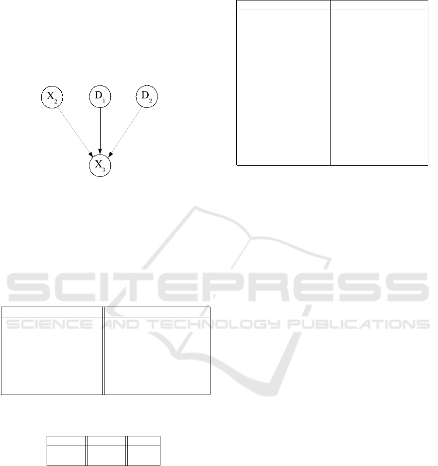
Using Algorithm 2, the graphical component G

will be deﬁned on set of variables Z = Par(V

) =

, X

, D

}. As already mentioned, an arbitrary

node must be selected from Z to be a child of the

remaining parent variables. The choice of this node

must be in accordance with the topological ordering

On the Decomposition of Min-based Possibilistic Inﬂuence Diagrams

123

induced by the reduced Inﬂuence Diagram. First, we

give the topological ordering induced by the reduced

Inﬂuence Diagram (Figure 3 ):

≺ X

≺ D

≺ X

Then, two nodes are worn candidates for this choice:

or X

, let X

be this node. The graphical compo-

nent G

is given by Figure 4.

Figure 4: Preference-based possibilistic network.

The conditional possibility distribution µ(X

) associated to X

is deﬁned using Equation

11. The results are mentioned in Table 9. Possibility

distributions on other nodes {D

, D

, X

} are uniform

(see Table 10).

Table 9: Initial possibility distribution ΠP

min

on X

µ(X

| D

) X

µ(X

| D

)

.2 ¬x

¬x

.9 ¬x

¬x

¬d

.3 ¬x

¬d

¬x

.1 ¬x

¬d

¬x

¬d

.2 ¬x

¬d

¬x

.2 ¬x

¬d

¬x

¬d

.3 ¬x

¬d

¬x

.3 ¬x

¬d

¬x

Table 10: Initial possibility distribution ΠP

min

on D

, D

and X

µ(D

) D

µ(D

) X

µ(X

)

1 d

1 x

¬d

1 ¬d

1 x

Using Equation 3, the preference-based possi-

bilistic network ΠP

min

induces the joint qualitative

utility µ

given by Table 11.

As illustrated by Tables 9 and 11, the conditional

possibility distribution µ(X

| D

) is the same as

the joint qualitative utility induced by the preferences-

based possibilistic network ΠP

min

. Therefore, we con-

clude that the proposed solution which consists in re-

ducing the initial Inﬂuence Diagram do not allow a

compact representation of agent’s preferences.

Table 11: The joint qualitative utility µ

, D

, X

.2 ¬d

¬x

.5 ¬d

¬x

.1 ¬d

¬x

.1 ¬d

¬x

.2 ¬d

¬x

.5 ¬d

¬x

.1 ¬d

¬x

.1 ¬d

¬x

¬d

.3 ¬d

¬d

¬x

0 ¬d

¬d

¬x

¬d

¬x

.1 ¬d

¬d

¬x

¬d

¬x

0 ¬d

¬d

¬x

¬d

¬x

.3 ¬d

¬d

¬x

¬d

¬x

0 ¬d

¬d

¬x

¬d

¬x

.1 ¬d

¬d

¬x

¬d

¬x

0 ¬d

¬d

¬x

3.2.2 Decomposition Process based on the Initial

Inﬂuence Diagram

The main limitation of the ﬁrst solution, presented in

Section 3.2.1 and inspired from the work proposed in

(Guezguez, 2012), concerns the reduction of all util-

ity nodes into a single one that will inherit the parents

of all value nodes. So, we suggest to preserve the ini-

tial structure. The solution proposed in this section

is to try to have the structure of a preference-based

network as close as possible to the initial structure of

the Inﬂuence Diagram. Hence, as we will see, oper-

ating on the initial structure of the Inﬂuence Diagram

allows a more compact representation than if we have

used the reduced Inﬂuence Diagram.

The min-based possibilistic network ΠP

min

, µ) encoding agent’s preferences is built progres-

sively as follows:

• For each utility node V

∈ V = {V

, ...,V

}, de-

ﬁne an order between parent variables. More pre-

cisely, this order is induced by the DAG associ-

ated with the initial Inﬂuence Diagram.

Example 4. Let us consider the Inﬂuence Dia-

gram given in Example 1 Figure 1. The parent

variables of utility node V

are D

and X

. We

recall that the Inﬂuence Diagram ΠID

min

induces

the following order:

≺ X

≺ D

≺ X

Then, an order can be deﬁned between parent

variables D

and X

as follows:

≺ X

• For each utility node V

∈ V = {V

, ...,V

}, a set

of nodes is deﬁned, among the parent variables of

where each node is eligible to be a child of the

ICAART 2016 - 8th International Conference on Agents and Artiﬁcial Intelligence

124

remaining parent variables. The candidate nodes

are those that appear in the last row of the order

list generated in the previous step. Indeed, re-

specting the order induced between the parents of

each utility node enables us to avoid the creation

of loops at the merging step of the evaluation pro-

cess (Benferhat et al., 2013). Each candidate node

can have one of the three following status:

1. Either it has not yet been introduced in the DAG

under construction.

2. Or it represents a root node in the DAG part

already built.

3. Or it represents a child.

• One node, denoted Z

must be selected from the

candidate set generated in the previous step. For

more compact representation of the DAG G

un-

der construction, the selected node must satisfy as

a priority the ﬁrst or second property (not yet in-

troduced or root node). If the selected node Z

not yet appear in the DAG G

under construction,

then we must ﬁrst integrate it in G

. In the same

way, parent variables that have not yet been inte-

grated in G

must be created. Finally, arcs from

the remaining parent variables to Z

must be cre-

ated.

If the selected node Z

already appears in the DAG

under construction as a root node, then we

must only integrate the remaining parent variables

that are not yet included in G

and create arcs

from the remaining parent variables to Z

Then, we proceed to compute the conditional pos-

sibility distribution µ(Z

| U

). In both situations

(1 or 2), the conditional possibility distribution

µ(Z

| U

) associated to the node Z

is deﬁned

as follows:

∀z

∈ D

, ∀u

∈ D

Par(Z

)

µ(z

| u

) = µ

). (13)

If such a node does not exist (all candidate nodes

are already children), then we choose the node

with a minimum number of parents in order to

have more compact representation. The condi-

tional possibility distribution µ(Z

| U

) associ-

ated to the node Z

is deﬁned as follows:

∀z

∈ D

, ∀u

∈ D

Par(Z

)

µ(z

| u

) = min[µ(z

| u

), µ

)]. (14)

• For each node Z

different from the selected node

will be associated a total ignorance possibility

distribution, namely:

∀z

∈ D

, µ(z

) = 1. (15)

The construction of preference-based possibilistic

network ΠP

min

can be summarized by Algorithm 3.

The proposed algorithm generates the qualitative

min-based possibilistic network ΠP

min

= (G

, µ) step

by step. Indeed, for each utility node, the algorithm

selects the candidate parents that can be a child of the

remaining parents in the DAG G

under construction.

These candidate nodes appear in the last rank of the

topological ordering generated by the ID. Among the

candidates, if there exists a node that has not yet been

introduced in G

or it presents a root node, so it will

be selected as the child of the remaining parent vari-

ables in the DAG G

under construction. Otherwise,

if such node does not exist then it means that all candi-

date nodes are already integrated in the DAG G

and

Data: {V

, Par(V

)}, ..., {V

, Par(V

)}, utility nodes

and their parents in the qualitative inﬂuence

diagram.

Result: ΠP

min

= (G

, µ), preference-based

possibilistic network.

begin

Z ←

0. /* Set of integrated variables in G

Child ←

foreach V

∈ {V

, ...,V

} do

List − order(V

) ← {Par(V

)} ordered in

the same way that the order induced by

ΠID

min

Candidate(V

) ← { the variables with the

last rank in the List − order(V

)}.

Select a variable Z

∈ Candidate(V

) and

6∈ Child.

if Z

exists then

Child ← Child ∪ {Z

}./*Z

presents

child in G

Create nodes Par(V

) 6∈ Z./*creating

nodes that not appear in G

Create arcs from {Par(V

) − Z

} to

./*creating arcs from the remaining

parent variables to the selected node

Quantifying chance node Z

using

Equation 13

else

Select a variable Z

∈ Candidate(V

)

and |Par(Z

)| in G

is the smallest.

Create nodes Par(V

) 6∈ Z.

Create arcs from {Par(V

) − Z

} to Z

Quantifying chance node Z

using

Equation 14

end

foreach Z

∈ Par(V

) and Z

6= Z

if Z

6∈ Child then

Quantifying chance node Z

using

Equation 15

end

Algorithm 3: Preference-based possibilistic network.

On the Decomposition of Min-based Possibilistic Inﬂuence Diagrams

125

they have parents (they present child). According to

the selected node status (not integrated, root or child)

an utility will be associated to this node. A total igno-

rance possibility distribution will be associated with

the remaining parent variables.

It is evident that the last solution which operates

on the initial ID structure (which does not require the

reduction of utility nodes to a single utility one) al-

lows a compact representation of the qualitative util-

ity.

It should be noted that in the case of an ID with

multiple utility nodes having no common parents,

the preference-based qualitative possibilistic network

will in fact be disconnected. Indeed, each component

of the graph encodes local satisfaction degrees asso-

ciated to one utility node.

The following proposition shows that the qualitative

possibilistic network ΠP

min

= (G

, µ), built follow-

ing the previous steps, encodes the same qualitative

utility encoded by the qualitative Inﬂuence Diagram

ΠID

min

, π

min

, µ

min

Proposition 3. Let ΠID

min

, π

min

, µ

min

) be a min-

based PID. Let ΠP

min

= (G

, µ) be a preferences-

based possibilistic network obtained using Algorithm

3. The joint qualitative utility µ

induced by ΠP

min

equal to the one induced by ΠID

min

. Namely,

, ..., Z

) = µ

min

, ..., X

, D

, ..., D

). (16)

4 RELATED WORKS

In possibilistic framework, few works exist on deci-

sion making. A possibilistic adaptation of the well

known ID has been proposed in (Garcia and Sab-

badin, 2006) (Guezguez et al., 2009) (Zhang, 2013),

etc. Both knowledge and utilities are described in

a same graphical structure using ordinal data. Like

the probabilistic ID, the PID

contain three types of

nodes: chance, decision and utility nodes. Uncer-

tainty is described by means of possibility distribu-

tions on chance nodes and preferences are expressed

as satisfaction degrees on utility nodes. To compute

optimal decisions, two methods have been proposed

in literature for evaluating qualitative PID: direct and

an indirect once. A direct method uses initial struc-

tures but require additional computations in order to

update possibility distribution tables (Garcia and Sab-

badin, 2006). Also, in (Garcia and Sabbadin, 2006),

an indirect method has been proposed which consists

to transform a PID into a decision tree. Recently, in

(Guezguez et al., 2009) a new indirect method has

been proposed to evaluate PID based on the transfor-

mation of this latter into qualitative possibilistic net-

work. It should be noted that the proposed solution

reduces utility nodes in a single one. On this new

structure the inference process will be made.

Recently in (Benferhat et al., 2013), authors have

proposed a new possibilistic graphical model for han-

dling decision problems under uncertainty. The pro-

posed solution for representing decision making un-

der uncertainty is based on the use of min-based pos-

sibilistic networks. It suggested to encode agent’s

knowledge and preferences by two distinct qualitative

possibilistic networks. The ﬁrst one encodes a joint

possibility distribution representing available knowl-

edge and the second one encodes the qualitative util-

ity. This new representation is in agreement with the

semantic deﬁnition of a qualitative decision problem

given in (Dubois et al., 1999). This new represen-

tation for decision making under uncertainty based

on min-based possibilistic networks, beneﬁts from the

simplicity of possibilistic networks. Indeed, the com-

putation of optimal decision is performed using infer-

ence process in a uniﬁed way. Unlike the solution pro-

posed in (Guezguez et al., 2009) for computing opti-

mal decisions, the decomposition process allows us to

obtain more compact representation. In fact, the pos-

sibilistic network issued from the fusion phase (Ben-

ferhat et al., 2013) is based on more compact repre-

sentation of the qualitative utility.

5 CONCLUSIONS

This paper concerns the decomposition of a Possi-

bilistic Inﬂuence Diagram into two possibilistic net-

works: the ﬁrst expresses agent’s knowledge and the

second encodes its preferences. This procedure al-

lows a simple representation of decision problems un-

der uncertainty. Indeed, the decomposition process

described in this paper offers a natural way to express

knowledge and preferences of a agent separately in

uniﬁed way using only one type of nodes. And in

order to perform the decomposition process, an algo-

rithm has been proposed and has conﬁrmed that the

new model based on the possibilistic networks (Ben-

ferhat et al., 2013) for representing decision making

has the capacity to encode any decision problem. The

proposed algorithm ensures a more compact represen-

tation of the graph used in evaluation phase for com-

puting optimal decisions.

As future work, we plan to extend the proposed

graphical model for the representation of decision

problems to deal with more complex problems involv-

ing sequential decisions. Indeed, one of the attractive

beneﬁts of Possibilistic Inﬂuence Diagrams consists

on their ability of dealing sequential decisions.

ICAART 2016 - 8th International Conference on Agents and Artiﬁcial Intelligence

126

ACKNOWLEDGEMENTS

This work has received supports from the french

Agence Nationale de la Recherche, ASPIQ project

reference ANR-12-BS02-0003. This work has also

received support from the european project H2020

Marie Sklodowska-Curie Actions (MSCA) research

and Innovation Staff Exchange (RISE): AniAge

(High Dimensional Heterogeneous Data based An-

imation Techniques for Southeast Asian Intangible

Cultural Heritage Digital Content), project number

691215.

REFERENCES

Ajroud, A., Omri, M., Youssef, H., and Benferhat, S.

(2012). Loopy belief propagation in bayesian net-

works : origin and possibilistic perspectives. CoRR,

abs/1206.0976.

Amor, N. B., Benferhat, S., Dubois, D., Mellouli, K., and

Prade, H. (2002). A theoretical framework for pos-

sibilistic independence in a weakly ordered setting.

International Journal of Uncertainty, Fuzziness and

Knowledge-Based Systems, 10(2):117–155.

Amor, N. B., Benferhat, S., and Mellouli, K. (2003). Any-

time propagation algorithm for min-based possibilis-

tic graphs. Soft Comput., 8(2):150–161.

Anzilli, L. (2013). A possibilistic approach to invest-

ment decision making. International Journal of Un-

certainty, Fuzziness and Knowledge-Based Systems,

21(02):201–221.

Benferhat, S., Khellaf, F., and Zeddigha, I. (2013). A pos-

sibilistic graphical model for handling decision prob-

lems under uncertainty. In The 8th conference of the

European Society for Fuzzy Logic and Technology,

EUSFLAT, Milano, Italy.

Borgelt, C., Gebhardt, J., and Kruse, R. (1998). Inference

methods. In Handbook of Fuzzy Computation, chapter

F1.2. Institute of Physics Publishing, Bristol, United

Kingdom.

Bouchon-Meunier, B., Coletti, G., and Marsala, C. (2002).

Independence and possibilistic conditioning. Annals

of Mathematics and Artiﬁcial Intelligence, 35:107–

123.

Boutouhami, K. and Khellaf, F. (2015). An approximate

possibilistic graphical model for computing optimistic

qualitative decision. In In proceedings of the Interna-

tional Conference on Artiﬁcial Intelligence and Appli-

cations AIFU, Dubai UAE, pages 183–196.

de Campos, M. L. and Huete, F. J. (1999). Indepen-

dence concepts in possibility theory. Fuzzy Sets Syst.,

103:487–505.

Denardo, E., Feinberg, E., and Rothblum, U. (2012). Split-

ting in a ﬁnite markov decision problem. SIGMET-

RICS Performance Evaluation Review, 39(4):38.

Dubois, D., Berre, D. L., Prade, H., and Sabbadin, R.

(1998). Logical representation and computation of op-

timal decisions in a qualitative setting. In AAAI-98,

pages 588–593.

Dubois, D., Fargier, H., and Prade, H. (2013). Decision-

making under ordinal preferences and comparative

uncertainty. CoRR, abs/1302.1537.

Dubois, D., Godo, L., Prade, H., and Zapico, A. (1999).

On the possibilistic decision model: from decision un-

der uncertainty to case-based decision. International

Journal of Uncertainty, Fuzziness and Knowledge-

Based Systems, 7(6):631–670.

Dubois, D. and Prade, H. (1988). Possibility Theory: An

Approach to Computerized Processing of Uncertainty

. Plenum Press, New York.

Dubois, D. and Prade, H. (1995). Possibility theory as a

basis for qualitative decision theory. In Proceedings

of the 14th international joint conference on Artiﬁcial

intelligence - Volume 2, pages 1924–1930, San Fran-

cisco, CA, USA. Morgan Kaufmann Publishers Inc.

Dubois, D., Prade, H., and Sabbadin, R. (2001). Decision-

theoretic foundations of qualitative possibility the-

ory . European Journal of Operational Research,

128(3):459–478.

Garcia, L. and Sabbadin, R. (2006). Possibilistic inﬂuence

diagrams. In 17th European Conference on Artiﬁ-

cial Intelligence (ECAI’06), pages 372–376, Riva del

Garda, Italy. IOS Press.

Giang, P. and Shenoy, P. (2005). Two axiomatic approaches

to decision making using possibility theory. European

Journal of Operational Research, 162(2):450–467.

Guezguez, W. (2012). Possibilistic Decision Theory:

From Theoretical Foundations to Inﬂuence Diagrams

Methodology. Phd thesis, Paul Sabatier University,

France.

Guezguez, W., Amor, N. B., and Mellouli, K. (2009). Qual-

itative possibilistic inﬂuence diagrams based on qual-

itative possibilistic utilities. European Journal of Op-

erational Research, 195(1):223–238.

Howard, R. and Matheson, J. (1984). Inﬂuence Diagrams.

In Readings on the Principles and Applications of De-

cision Analysis, pages 721–762. Strategic Decisions

Group.

Huang, C. and Darwiche, A. (1996). Inference in belief net-

works: A procedural guide. Int. J. Approx. Reasoning,

15(3):225–263.

Lauritzen, S. and Nilsson, D. (2001). Representing and

solving decision problems with limited information.

Manage. Sci., 47(9):1235–1251.

Shenoy, P. (1994). A comparison of graphical techniques

for decision analysis. European Journal of Opera-

tional Research, 78:1–21.

Sniedovich, M. (2010). Dynamic Programming: Founda-

tions and Principles; 2nd ed. Pure and Applied Math-

ematics. CRC Press, Hoboken.

Tatman, J. and Shachter, R. (1990). Dynamic programming

and inﬂuence diagrams. IEEE Transactions on Sys-

tems, Man and Cybernetics, 20(2):365–379.

Whalen, T. (1984). Decision making under uncertainty

with various assumptions about available informa-

tion. IEEE Trans. on systems, Man and Cybernetics,

(14):888–900.

On the Decomposition of Min-based Possibilistic Inﬂuence Diagrams

127

Zadeh, L. (1978). Fuzzy sets as a basis for a theory of pos-

sibility. Fuzzy Sets and Systems, 1:3–28.

Zhang, N. (1998). Probabilistic inference in inﬂuence di-

agrams. In Computational Intelligence, pages 514–

522.

Zhang, N. (2013). Probabilistic inference in inﬂuence dia-

grams. CoRR, abs/1301.7416.

ICAART 2016 - 8th International Conference on Agents and Artiﬁcial Intelligence

128