
Understanding the Interplay of Simultaneous Model Selection and
Representation Optimization for Classification Tasks
Fabian B¨urger and Josef Pauli
Intelligent Systems Group, University of Duisburg-Essen, Bismarckstraße 90, 47057 Duisburg, Germany
Keywords:
Model Selection, Representation Learning, Classification, Evolutionary Optimization.
Abstract:
The development of classification systems that meet the desired accuracy levels for real world-tasks appli-
cations requires a lot of expertise. Numerous challenges, like noisy feature data, suboptimal algorithms and
hyperparameters, degrade the generalization performance. On the other hand, almost countless solutions have
been developed, e.g. feature selection, feature preprocessing, automatic algorithm and hyperparameter selec-
tion. Furthermore, representation learning is emerging to automatically learn better features. The challenge
of finding a suitable and tuned algorithm combination for each learning task can be solved by automatic opti-
mization frameworks. However, the more components are optimized simultaneously, the more complex their
interplay becomes with respect to the generalization performance and optimization run time. This paper an-
alyzes the interplay of the components in a holistic framework which optimizes the feature subset, feature
preprocessing, representation learning, classifiers and all hyperparameters. The evaluation on a real-world
dataset that suffers from the curse of dimensionality shows the potential benefits and risks of such holistic
optimization frameworks.
1 INTRODUCTION
Classifier systems learn the connection between fea-
ture data and class labels and are potentially useful in
many applications such as image-based object recog-
nition, automated quality inspection and medical di-
agnosis systems. The development of classifier sys-
tems for real-world tasks is still challenging, even
though many sophisticated classifiers, such as Sup-
port Vector Machines (SVM) or random forests, ex-
ist. The reasons for this are manifold: At first, the
input feature data can be noisy, especially when raw
sensor data is used, like pixel data from camera sen-
sors. The development of task-specific features which
are invariant to certain variations is time-consuming
and requires a lot of expertise. Secondly, there is no
best performing general-purpose machine learning al-
gorithm and so a suitable one has to be chosen. Fur-
thermore, most algorithms have hyperparameters that
need to be adapted to each learning task.
Many well known, established solutions to almost
all of these challenges exist, like feature selection al-
gorithms, feature preprocessing methods or automatic
algorithm and hyperparameter selection methods.
The field of representation learning aims at im-
proving the feature data and it has shown a great per-
formance boost in e.g. deep learning (Bengio et al.,
2013). The goal is to automatically generate better
suitable features out of low-level data. One way of
learning a better representation is manifold learning
that results in easier and lower dimensional features
(Ma and Fu, 2011).
The large number of potentially useful approaches
makes it difficult to select the optimal algorithm com-
bination for each learning task. This challenge has
motivated the development of automatic optimization
frameworks that can handle a great amount of solu-
tions. Currently, there are two promising optimiza-
tion approaches to tackle the highly combinatorial
so-called algorithm configuration problem. The first
approach is Evolutionary Optimization (B¨ack, 1996)
which simulates the natural evolution process. It has
been successfully used to select features and classifier
hyperparameters(Huang and Chang, 2007; Ans´otegui
et al., 2009), also in combination with manifold learn-
ing (B¨urger and Pauli, 2015). The second approach
is Bayesian optimization (Snoek et al., 2012; Hutter
et al., 2011) that collects all information about the
optimization trajectory in a probabilistic model and
evaluates the next most promising areas of the search
space. The Auto-WEKA framework (Thornton et al.,
2013) uses this approach to optimize features, algo-
Bürger, F. and Pauli, J.
Understanding the Interplay of Simultaneous Model Selection and Representation Optimization for Classification Tasks.
DOI: 10.5220/0005705302830290
In Proceedings of the 5th International Conference on Pattern Recognition Applications and Methods (ICPRAM 2016), pages 283-290
ISBN: 978-989-758-173-1
Copyright
c
2016 by SCITEPRESS – Science and Technology Publications, Lda. All rights reserved
283

rithms and hyperparameters.
These holistic frameworks are successful, but the
large degree of adaptability of the optimized classi-
fier systems can cause overfitting that degrades the
generalization performance. Therefore, a deeper un-
derstanding of the interplay of the involved optimiza-
tion components is necessary. This paper quantifies
the impact of feature selection, feature preprocessing,
manifold and representation learning, classifier selec-
tion and hyperparameter tuning on generalization per-
formance and optimization time using an Evolution-
ary Algorithm. Furthermore, three aspects regarding
the optimization algorithm itself are analyzed as well.
This paper is organized as follows. Section 2
lists a selection of approaches to improve machine
learning. Section 3 presents a holistic classification
framework that incorporates these aspects. Section
4 discusses the Evolutionary Optimization strategy
to adapt the algorithm configuration to each learning
task. Section 5 presents the results of the evaluation
of the framework. Finally, section 6 contains the con-
clusions.
2 MACHINE LEARNING
SOLUTIONS
This section discusses approaches to improve ma-
chine learning subdivided into established methods
and representation learning.
2.1 Established Approaches
There are some very popular “standard” approaches
to improve the performance of machine learning sys-
tems, which are described in e.g. (Jain et al., 2000) or
(Bishop and Nasrabadi, 2006).
Feature selection algorithms have the goal to
choose a useful subset of features to remove irrelevant
and noisy dimensions. Feature selection is a remedy
to the curse of dimensionality. Feature preprocess-
ing methods are relatively simple algorithms that e.g.
normalize the value ranges of the features to a defined
range or remove correlations between features which
is known as pre-whitening (Juszczak et al., 2002).
Model selection algorithms have the goal to se-
lect an optimal classification model for a specific task.
This can comprise the selection of a specific algo-
rithm out of an portfolio of alternatives and the tun-
ing of hyperparameters. The best performing model
is usually determined by generalization estimation
based on model validation techniques such as cross-
validation.
2.2 Representation Learning
The development of task-specific features can be one
of the most time-consuming parts of the development
process. The field of automatic feature construction
methods is one part of representation learning and
aims at automatically learn better feature representa-
tions out of the provided data. The family of man-
ifold learning methods provides such functionality –
examples are Principal Component Analysis (PCA),
Isomap, Local Linear Embedding (LLE) or Autoen-
coders. References to these methods can be found
e.g. in (Van der Maaten et al., 2009) or (Ma and Fu,
2011). Most of these methods are unsupervised and
thus do not require expensive, labeled ground truth
data. However, the success of these methods depends
on the datasets. Furthermore, not all methods provide
a so-called direct out-of-sample extension that em-
beds unseen instances into the learned feature space,
butonly an approximationwhich can degrade the gen-
eralization performance.
3 HOLISTIC CLASSIFICATION
FRAMEWORK
The classification pipeline is similar to our previ-
ous work (B¨urger and Pauli, 2015) and incorporates
all approaches discussed in section 2 into a holistic
framework. The pipeline consists of four pipeline el-
ements and is depicted in figure 1. The originally
proposed “feature scaling” element is replaced by a
generalized preprocessing element. The pipeline has
two modes, namely the training and classification
mode. The training mode is used to adapt and train
the pipeline configuration θ using the training dataset
T. This training dataset T = {(x
1
, y
1
), . . . , (x
m
, y
m
)} is
the input of the frameworkand contains m labeled fea-
ture vectors x
i
∈ R
D
in
and corresponding class labels
y
i
∈ {ω
1
, ω
2
, . . . , ω
c
}. The classification mode uses a
specific configuration to set up a pipeline which pro-
cesses the incoming feature vectors and returns class
labels. The functionality of each pipeline element is
described in the following.
3.1 Feature Selection Element
The first element contains the functionality of feature
selection to remove irrelevant features as soon as pos-
sible. A feature subset S
FeatSet
∈ P ({1, 2, ..., D
in
}) \
/
0
is selected during the training mode. In the classifi-
cation mode, the determined subset of dimensions is
selected from the incoming features vectors and the
ICPRAM 2016 - International Conference on Pattern Recognition Applications and Methods
284
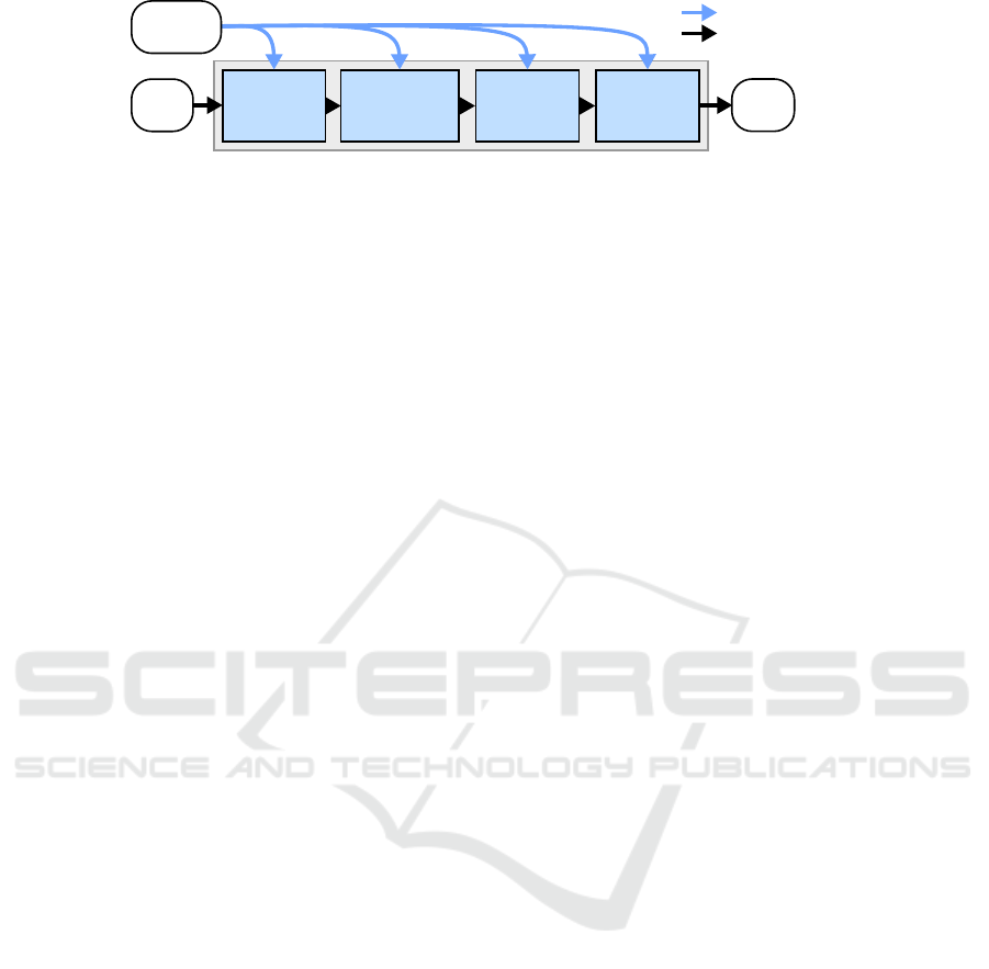
Feature
Preprocessing
Element
Feature
Transform
Element
Input
vector
Class
label
Classifier
Element
Feature
Selection
Element
Training
dataset
Classification Mode
Training Mode
Figure 1: Classification pipeline structure and data processing in the training and classification mode.
others are removed. The feature dimensionality is de-
creased according to the number of selected features
|S
FeatSet
|.
3.2 Feature Preprocessing Element
The second pipeline element contains the function-
ality of feature preprocessing to provide better us-
able features for the learning algorithms in the next
two pipeline elements. This pipeline element has a
portfolio of preprocessing algorithms S
PreProc
which
contains four methods, namely feature rescaling of
each dimension to a range of [0, 1], statistical stan-
dardization, L
2
normalization, pre-whitening and –
additionally – the identity. In the training mode one
method f
PreProc
∈ S
PreProc
is chosen. In the classifi-
cation mode, the selected preprocessing is applied to
the incoming feature vectors.
3.3 Feature Transform Element
The third element introduces the aspect of represen-
tation learning into the classification pipeline. This is
realized in form of feature transforms that are learned
using manifold learning techniques. The pipeline el-
ement contains a portfolio S
FeatTrans
with 32 mani-
fold learning techniques provided by the Matlab Tool-
box for Dimensionality Reduction (Van der Maaten,
2014). Additionally, similar to the feature prepro-
cessing method, the identity is included, too. In
the training mode a method f
FeatTrans
∈ S
FeatTrans
as
well as values for the specific set of hyperparameters
S
Hyp
( f
FeatTrans
) are chosen. Additionally, the target
dimensionality D
Target
of the resulting feature space
needs to be chosen which is a common hyperparame-
ter of all manifold learners. Then the manifold learner
is trained with the feature vectors arriving from the
feature preprocessing element. Most manifold learn-
ing algorithms are unsupervised, but the supervised
ones additionally use the corresponding labels from
the training dataset T. In the classification mode, the
out-of-sample extension or approximation of the se-
lected and trained manifold learner is applied to pro-
cess the feature vectors.
3.4 Classifier Element
The fourth pipeline element is finally responsible to
perform the actual classification. The pipeline ele-
ment contains a portfolio S
Classifiers
of eight popular
classifier concepts and variants, e.g. kernel Support
Vector Machines (SVM), random forests and the mul-
tilayer perceptron. In the training mode, a classifier
concept f
Classifier
∈ S
Classifiers
is selected as well as its
specific set of hyperparameters S
Hyp
( f
Classifier
). The
classifier is trained using the processed feature vectors
and the corresponding labels in the training dataset T.
In the classification mode, the trained classifier is used
to classify instances.
3.5 Pipeline Configuration
The pipeline configuration contains all necessary in-
formation about the selected features, algorithms and
hyperparameters and is defined as
θ = (S
FeatSet
, f
PreProc
, f
FeatTrans
, S
Hyp
( f
FeatTrans
),
D
Target
, f
Classifier
, S
Hyp
( f
Classifier
)). (1)
The number of possible configurations is huge and
also depends on the training dataset, because there are
2
D
in
− 1 possible feature subsets to choose from.
4 OPTIMIZATION FRAMEWORK
The pipeline configuration θ needs to be adapted to
every learning task defined by the training dataset T.
An optimization algorithm is required that can han-
dle the large search space which will likely also con-
tain a large number of local optima. Evolutionary Al-
gorithms have the potential to cope with these chal-
lenges and it is known that they can be easily run in
parallel – which is not the case for a Bayesian opti-
mization approach.
4.1 Extended Evolution Strategies
Evolution Strategies (ES) (Beyer and Schwefel, 2002)
are one variant of Evolutionary Algorithms which are
Understanding the Interplay of Simultaneous Model Selection and Representation Optimization for Classification Tasks
285
suitable to solve high-dimensional optimization prob-
lems. A solution is coded into the genetic information
of an individual and a population contains several in-
dividuals. Starting from an initial population which
is usually generated randomly, the best individuals
are selected according to their fitness. The fitness is
usually determined using the objective function of the
optimization problem (see section 4.3). The selected
individuals are recombined and randomly mutated to
generate a new generation of hopefully improved in-
dividuals. This procedure is repeated until the termi-
nation criteria are fulfilled, e.g. too little fitness im-
provements or a time limit.
The standard ES is only defined for numeric vari-
ables, but all necessary evolutionary operators can be
extended to more data types which is described by
the authors of (B¨urger and Pauli, 2015). The config-
uration adaption problem requires a larger variety of
variable types, because of the feature selection and
hyperparameter tuning problem. Therefore, the fol-
lowing variable types are used:
• The real-valued variable type V
R
,
• the integer variable type V
Z
,
• the categorical variable type V
S
and
• the Boolean variable type V
B
.
The numeric variables also contain information
about minimum and maximum values and the cat-
egorical variables the base set of all possible cate-
gories.
The parametrization of an ES-based optimization
algorithm is summarized in the (µ, κ, λ, ρ) notation. In
each generation λ = 200 individuals from ρ = 3 par-
ents are generated while the best µ = 20 individuals
survive. The maximum lifespan of individuals is lim-
ited to κ = 4 generations. The initial population con-
tains µ
init
= 400 random individuals. The number of
individuals should be as high as possible to increase
the chances to find better solutions. However, there
must be a trade-off between computational complex-
ity and the risk of getting stuck in local optima.
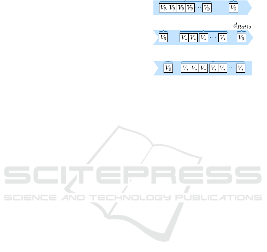
4.2 Evolutionary Configuration
Adaptation
The pipeline configurations have to be coded into the
genotype of the ES which is a sequence of N variables
G = [V
∗,1
,V
∗,2
, . . . ,V
∗,N
], V
∗
∈ {V
R
,V
Z
,V
S
,V
B
}. (2)
The Evolutionary Configuration Adaption (ECA)
schema is used to code a configuration into the geno-
type as depicted in figure 2. First, the feature selec-
tion problem is coded as D
in
binary variables that in-
dicate whether a feature is selected or not. The feature
Feature
preprocessing
Feature
transform
Feature transform
hyperparameters
Classifier
Classifier
hyperparameters
Feature
subset
Figure 2: ES genotype coding schema of a pipeline config-
uration.
preprocessing method is coded as a single categorical
variable. The feature transform is also selected with
a categorical variable. All hyperparameters of all fea-
ture transforms are also appended to the genome with
their corresponding variable type. When the individ-
uals are transformed to a configuration, only those
hyperparameters are used that belong to the selected
feature transform. The target dimensionality depends
on the number of selected features and therefore it is
coded as a real-valued ratio d
Ratio
∈ [0, 1]. The actual
value for the target dimensionality is then calculated
as D
Target
= ⌊d
Ratio
·|S
FeatSet
|⌋. The classifier is coded
similarly to the feature transform as categorical vari-
able and the corresponding hyperparameters are also
handled in the same way. Each individual I can be
mapped to a valid pipeline configuration θ.
4.3 Fitness Function
The key role of ES is the selection of individuals
I by their fitness fit(I). In case of a classification
pipeline, the fitness should be directly connected to
the expected generalization performance of the whole
pipeline. Therefore, a holistic k-fold cross-validation
(HCV) is used that considers the generalization of all
components. This is necessary, because especially the
feature transform is expected to contribute to the gen-
eralization.
The HCV method uses the training dataset T
to generate k = 5 disjoint training and validation
tuples {(T
train,l
, T
valid,l
)} with 1 ≤ l ≤ k. In each
cross-validation round, the classification pipeline is
first trained using T
train,l
. Subsequently, the instances
of the validation dataset T
valid,l
are classified with
this pipeline and the overall accuracy value q
acc,l
is
calculated. This makes sure that the validation data is
never used for training. During the cross-validation
process, the average overall accuracy so far
ICPRAM 2016 - International Conference on Pattern Recognition Applications and Methods
286

q
acc,l
=
1
l
l
∑
j=1
q
acc, j
(3)
is calculated. This value is used for an early dis-
carding system to save computation time. The cross-
validation process is stopped prematurely for bad per-
forming configurations that do not improve the pre-
viously observed best accuracy value q
∗
acc
. The early
discarding system is relatively aggressive and the pro-
cess is stopped if
q
acc,l
< q
∗
acc
. The last average is
used as fitness value for the individuals fit(I) = q
acc,l
.
This fitness metric is also used as termination cri-
terion. The optimization is stopped when the best
fitness of the current generation increases less than
ε = 10
−3
(equal to 0.1 percent of accuracy) over the
last three generations.
4.4 Initial Population Improvement
The feature selection problem is expected to have
the largest impact on the problem complexity and
therefore, it is promising to speedup and improve
the ES optimization with an improved initial pop-
ulation. Random forests (Breiman, 2001) provide
an integrated feature importance metric proposed by
(Genuer et al., 2010). Before the actual ES optimiza-
tion begins, this metric β
i
is calculated for each fea-
ture with 1 ≤ i ≤ D
in
. The initial probability for each
feature is determined by the importance metric using
p
i
= p
min
+ (1− p
min
)
β
i
− β
min
β
max
− β
min
∈ [p
min
, 1] (4)
in which β
min
and β
max
are the minimum and maxi-
mum values of β
i
across all features. The p
min
= 0.25
value defines a minimum probability value for the
least important variable. This makes sure that the se-
lection of this variable does not become impossible.
4.5 Optimization Algorithm Variants
One of the main goals of this paper is to quantify and
understand the impact of the components of the clas-
sification pipeline. This is achieved by the introduc-
tion of restricted variants of the ECA optimization al-
gorithm that work with the leave-one-out principle for
each component. The following variants are consid-
ered:
• The ECA-full variant uses all components,
• the ECA-noFeatSel variant does not consider fea-
ture selection and always uses the full feature sub-
set,
• the ECA-noPreProc variant does not use any fea-
ture preprocessing method,
Figure 3: Three example images from each class of the
coins dataset.
• the ECA-noTrans variant does not use manifold
learning or feature transform methods,
• the ECA-simpleClassifier variant only contains a
simple classifier, namely the naive Bayes classi-
fier and
• the ECA-defaultHyper variant does not consider
hyperparameter tuning and leaves all hyperparam-
eters at their standard values.
5 EVALUATION
An image-based object recognition task is used to
evaluate the components of the framework. The task
is to classify color images of five classes of Euro coins
which are depicted in figure 3. There are 64 color im-
ages from 1-, 2-, 5-, 10- and 20-cent coins leading to
320 images in total. The following feature set is ex-
tracted from each image:
• The object area in pixels,
• statistical features of the gray value and color
channel histogram,
• Hu moments of the gray value texture (Hu, 1962),
• Local Binary Patterns (Ojala et al., 2002) of the
gray value texture,
• low-level pixel features in form of down-scaled
gray value images: 5 × 5, 10 × 10, and 20 × 20
pixels.
The total dimensionality of the feature space is D
in
=
642. In combination with the small number of sam-
ples negative effects due to the curse of dimensional-
ity can be expected. However, this makes this dataset
particularly interesting to analyze. The dataset is sep-
arated randomly into 50 % training and 50 % test
dataset.
The reported cross-validation accuracy is ob-
tained on the training dataset and is equal to the fit-
ness of the best individual. The generalization per-
formance is measured by using the configuration with
Understanding the Interplay of Simultaneous Model Selection and Representation Optimization for Classification Tasks
287

the highest fitness value to set up a classification
pipeline and process and evaluate the test dataset with
it. The optimization time is measured as well.
The performance of the ECA strategy is com-
pared to two baseline methods, namely an SVM clas-
sifier with a Gaussian kernel (denoted as Baseline-
SVM) and a random forest (denoted as Baseline-RF).
The baselines also use a grid-based hyperparameter
tuning with cross-validation. Furthermore, the per-
formance of the Auto-WEKA framework (Thornton
et al., 2013) with a time budget of 24 hours is com-
pared as well. Each experiment with the framework
is repeated ten times to obtain statistically relevant
results. All performance metrics are compared rel-
atively to the ECA-full strategy using a Welch test
1
(Howell, 2006) with a level of significance of α =
0.05 to show if the deviations are statistically signifi-
cant. If this is the case, the corresponding results are
marked with an exclamation mark.
The framework is implemented in Matlab 2014b
using the parallel computing toolbox and is running
on a workstation computer with 6 × 2.5Ghz and
32GB of RAM.
5.1 Results using All Components
The ECA-full variant of the framework can use the
full potential of all pipeline elements and is there-
fore the most promising and interesting approach.
Table 1 shows the results regarding the accuracy
values and optimization times. The two baseline
methods, especially the SVM, perform badly on this
dataset. An explanation is that this dataset suffers
from the curse of dimensionality. The ECA-full vari-
ant shows much higher cross-validation and gener-
alization accuracy values which also outperform the
Auto-WEKA framework significantly.
The typical processing time of the ECA-full strat-
egy stays under two hours. The two baseline methods
are much faster, because these are simple classifiers
which just undergo a grid search for the best hyperpa-
rameters. The Auto-WEKA framework uses its time
budget of 24 hours to optimize and does not prema-
turely stop.
5.2 Impact of the Pipeline Components
The ECA-full variant provides the greatest amount
of adaptability and performs well, but it is impor-
tant to understand the contribution of the classifica-
tion pipeline components. Figure 4 shows the impact
1
The Welch test is a statistical method to show if the
means of two samples are significantly different while no
assumptions about the sample variances are made.
of the pipeline components on the accuracy and the
optimization times by comparing the restricted ECA
variants (see section 4.5) to the ECA-full variant.
All restricted variants of the ECA strategy show
worse average accuracy values than the ECA-full vari-
ant (see the left side of figure 4). This observation
affects the cross-validation and the generalization ac-
curacy values. All differences, except of the cross-
validation accuracy of the ECA-defaultHyper variant,
are also statistically significant. The classifier port-
folio has the largest impact here, because the ECA-
simpleClassifier variant which uses only the Bayes
classifier achieves around 15 % less generalization ac-
curacy on average. The other components are obvi-
ously not able to compensate a too simple classifier.
The impact of the other components is smaller, but
still significant. It is interesting that the feature pre-
processing has a slightly larger impact than the feature
transforms, because the ECA-noPreProc variant per-
forms worse than the ECA-noTrans variant. This in-
dicates that relatively simple preprocessing methods
can lead to more improvement than 32 highly nonlin-
ear manifold learning methods.
The hyperparameter tuning component has a rela-
tively small impact on the accuracy values. It is likely
the case that – by chance – the standard hyperparam-
eters already work reasonably well for the dataset.
Also the aspect of feature selection is less important
here, because the accuracy values drop only about 1 -
2 % if feature selection is switched off.
The different pipeline components also affect the
average processing times (see the right side of fig-
ure 4) and most of the differences are statistically
significant. The use of feature selection speeds up
the optimization tremendously by more then 50 min-
utes on average, because a lower dimensional fea-
ture space requires less computation time for most
of the involved algorithms. The use of feature trans-
forms slows down the optimization process by almost
50 minutes on average. This can be explained with
the computationally complex models of the manifold
learning algorithms, but also their potentially experi-
mental implementation within Matlab. The use of the
feature preprocessing methods also slows down the
optimization process by more than 20 minutes on av-
erage. But the reason is not the computational com-
plexity of the preprocessing methods – which are sim-
ple actually –, but that more complex feature trans-
forms and classifiers perform better on preprocessed
features and therefore are chosen more often in the
ES optimization. Another reason is the larger search
space. A similar explanation can be found to justify
the same effect when hyperparameter tuning is active.
ICPRAM 2016 - International Conference on Pattern Recognition Applications and Methods
288
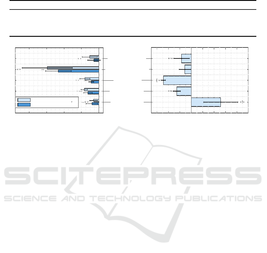
Table 1: Comparison of cross-validation and generalization accuracy results as well as optimization times (mean ±1σ).
Cross-validation acc. Generalization acc. Optimization time [min]
ECA-full 0.935 ± 0.015 0.951 ± 0.013 73.74 ± 20.28
Baseline-SVM 0.119 ± 0.013 (!) 0.281 ± 0.020 (!) 0.02 ± 0.01 (!)
Baseline-RF 0.623 ± 0.028 (!) 0.708 ± 0.045 (!) 0.48 ± 0.01 (!)
Auto-WEKA (not comparable) 0.930 ± 0.014 (!) 1440 = 24 hours (!)
Accuracy change
-0.2 -0.15 -0.1 -0.05 0
Generalization accuracy
Cross-validation accuracy
Optimization time change [min]
-60 -40 -20 0 20 40 60 80 100
ECA-noFeatSel
ECA-noPreProc
ECA-noTrans
ECA-simpleClassifier
ECA-defaultHyper
(!)
(!)
(!)
(!)
(!)
(!)
(!)
(!)
(!)
(!)
(!)
(!)
(!)
Figure 4: Impact of the pipeline components on accuracy values and optimization times compared to the ECA-full variant.
The standard deviations are denoted as lines around the end of the bars.
5.3 Impact of the ECA Algorithm
In the following, the impact of three central aspects
of the ECA optimization algorithm are investigated
by switching off the corresponding component of the
ECA-full algorithm. Table 2 lists the results regarding
the accuracy values and the optimization times.
5.3.1 Impact of Holistic Cross-validation
Instead of HCV (see section 4.3), a classifier-only
cross-validation approach is used for this experi-
ment. The pipeline is trained using the full train-
ing dataset and only the classifier performs cross-
validation. With this procedure, the generalization
of the feature transform is never considered. This
leads to a cross-validation accuracy value of 100 %,
but the resulting generalization accuracy is unusably
bad. However, the average optimization time drops
slightly due to the reduced computational complexity
of the classifier-only cross-validation.
5.3.2 Impact of Early Discarding
The early discarding system is an aggressive system
to save computation time (see section 4.3). It can be
seen that the average computation time rises tremen-
dously by a factor of around 3.8 when the early dis-
carding system is not used. The system does not have
any significant positive or negative effect on the accu-
racy values.
5.3.3 Impact of Initial Population Improvement
The initial population improvement affects the feature
selection (see section 4.4). If there is no initial im-
provement and a completely random initialization of
the features is used, the cross-validation and general-
ization accuracy values drop significantly. The com-
putation time actually drops slightly, but not signifi-
cantly, if the initial population is not improved. It is
likely the case that the termination criterion of the ES
algorithm was fulfilled too early.
6 CONCLUSIONS
This paper analyzed the impact of multiple aspects
of a holistic model selection and representation opti-
mization framework on accuracy values and optimiza-
tion times. The first experiment analyzed the impact
of the components of the classification pipeline. It
was shown that all involved components, namely fea-
ture selection, multiple preprocessing methods, multi-
ple feature transforms, multiple classifiers and hyper-
parameter tuning are potentially contributing to the
generalization performance. However, multiple ob-
servations have been made that indicate that the inter-
play between the involved components is complex –
especially regarding the optimization run times. It can
be expected that some effects are highly dependent on
the dataset.
The second experiment analyzed the impact of
Understanding the Interplay of Simultaneous Model Selection and Representation Optimization for Classification Tasks
289

Table 2: Impact of the central components of the ECA optimization algorithm on the accuracy values and optimization times
(mean ±1σ).
Cross-validation acc. Generalization acc. Optimization time [min]
ECA-full 0.935 ± 0.015 0.951 ± 0.013 73.74 ± 20.28
No holistic cross-validation 1.000 ± 0.0 (!) 0.287 ± 0.022 (!) 59.95 ± 9.16
No early discarding system 0.938 ± 0.024 0.933 ± 0.027 276.15 ± 59.64 (!)
No initial population improvement 0.912 ± 0.022 (!) 0.925 ± 0.025 (!) 59.30 ± 14.95
three aspects of the optimization algorithm itself. At
first, it was shown that the incorporation of the feature
transform into the cross-validation process is abso-
lutely necessary. Secondly, the early discarding sys-
tem greatly improvesthe optimization speed while the
resulting accuracyvalues are not affected in a negative
way. And lastly, the incorporation of prior knowledge
about the importance of features into the optimization
algorithm improved the accuracy.
Ultimately, it can be concluded that not only the
amount of optimized components is important, but
also the suitability of the optimization algorithm it-
self. However, further experiments on other datasets
need to be conducted to explore the full variety of ef-
fects regarding the complex interplay of the machine
learning components.
REFERENCES
Ans´otegui, C., Sellmann, M., and Tierney, K. (2009). A
gender-based genetic algorithm for the automatic con-
figuration of algorithms. In Gent, I., editor, Principles
and Practice of Constraint Programming - CP 2009,
volume 5732 of Lecture Notes in Computer Science,
pages 142–157. Springer Berlin Heidelberg.
B¨ack, T. (1996). Evolutionary Algorithms in Theory and
Practice: Evolution Strategies, Evolutionary Pro-
gramming, Genetic Algorithms. Oxford University
Press, Oxford, UK.
Bengio, Y., Courville, A., and Vincent, P. (2013). Represen-
tation learning: A review and new perspectives. Pat-
tern Analysis and Machine Intelligence, IEEE Trans-
actions on, 35(8):1798–1828.
Beyer, H.-G. and Schwefel, H.-P. (2002). Evolution strate-
gies - a comprehensive introduction. Natural Comput-
ing, 1(1):3–52.
Bishop, C. M. and Nasrabadi, N. M. (2006). Pattern recog-
nition and machine learning, volume 1. Springer New
York.
Breiman, L. (2001). Random forests. Machine Learning,
45(1):5–32.
B¨urger, F. and Pauli, J. (2015). Representation optimiza-
tion with feature selection and manifold learning in a
holistic classification framework. In De Marsico, M.
and Fred, A., editors, ICPRAM 2015 - Proceedings of
the International Conference on Pattern Recognition
Applications and Methods, volume 1, pages 35–44,
Lisbon, Portugal. INSTICC, SCITEPRESS.
Genuer, R., Poggi, J.-M., and Tuleau-Malot, C. (2010).
Variable selection using random forests. Pattern
Recognition Letters, 31(14):2225 – 2236.
Howell, D. C. (2006). Statistical Methods for Psychology.
Wadsworth Publishing.
Hu, M.-K. (1962). Visual pattern recognition by moment
invariants. Information Theory, IRE Transactions on,
8(2):179–187.
Huang, H.-L. and Chang, F.-L. (2007). ESVM: Evolution-
ary support vector machine for automatic feature se-
lection and classification of microarray data. Biosys-
tems, 90(2):516 – 528.
Hutter, F., Hoos, H., and Leyton-Brown, K. (2011). Se-
quential model-based optimization for general algo-
rithm configuration. In Coello, C., editor, Learning
and Intelligent Optimization, volume 6683 of Lecture
Notes in Computer Science, pages 507–523. Springer
Berlin Heidelberg.
Jain, A. K., Duin, R. P. W., and Mao, J. (2000). Statistical
pattern recognition: a review. Pattern Analysis and
Machine Intelligence, IEEE Transactions on, 22(1):4–
37.
Juszczak, P., Tax, D., and Duin, R. (2002). Feature scal-
ing in support vector data description. In Proc. ASCI,
pages 95–102. Citeseer.
Ma, Y. and Fu, Y. (2011). Manifold Learning Theory and
Applications. CRC Press.
Ojala, T., Pietikainen, M., and Maenpaa, T. (2002). Mul-
tiresolution gray-scale and rotation invariant texture
classification with local binary patterns. Pattern Anal-
ysis and Machine Intelligence, IEEE Transactions on,
24(7):971–987.
Snoek, J., Larochelle, H., and Adams, R. P. (2012). Prac-
tical bayesian optimization of machine learning algo-
rithms. In Advances in neural information processing
systems, pages 2951–2959.
Thornton, C., Hutter, F., Hoos, H. H., and Leyton-Brown,
K. (2013). Auto-WEKA: Combined selection and
hyperparameter optimization of classification algo-
rithms. In Proc. of KDD-2013, pages 847–855.
Van der Maaten, L. (2014). Matlab Tool-
box for Dimensionality Reduction.
http://lvdmaaten.github.io/drtoolbox/.
Van der Maaten, L., Postma, E., and Van Den Herik, H.
(2009). Dimensionality reduction: A comparative re-
view. Journal of Machine Learning Research, 10:1–
41.
ICPRAM 2016 - International Conference on Pattern Recognition Applications and Methods
290
