Parallel Implementation of Spatial Pooler in Hierarchical Temporal

Memory

Marcin Pietron

1,2

, Maciej Wielgosz

1,2

and Kazimierz Wiatr

1,2

AGH University of Science and Technology, Mickiewicza 30, 30-059, Cracow, Poland

ACK Cyfronet AGH, Nawojki 11, 30-950, Cracow, Poland

Keywords:

Artiﬁcial Intelligence, GPGPU Computing, Hierarchical Temporal Memory, Machine Learning, Neocortex.

Abstract:

Hierarchical Temporal Memory is a structure that models some of the structural and algorithmic properties of

the neocortex. HTM is a biological model based on the memory-prediction theory of brain. HTM is a method

for discovering and learning of observed input patterns and sequences, building an increasingly complex mod-

els. HTM combines and extends approaches used in sparse distributed memory, bayesian networks, spatial

and temporal clustering algorithms, using a tree-shaped hierarchy neural networks. It is quite a new model of

deep learning process, which is very efﬁcient technique in artiﬁcial intelligence algorithms. HTM like other

deep learning models (Boltzmann machine, deep belief networks etc.) has structure which can be efﬁciently

processed by parallel machines. Modern multi-core processors with wide vector processing units (SSE, AVX),

GPGPU are platforms that can tremendously speed up learning, classifying or clustering algorithms based on

deep learning models (e.g. Cuda Toolkit 7.0). The current bottleneck of this new ﬂexible artifﬁcial intelli-

gence model is efﬁciency. This article focuses on parallel processing of HTM learning algorithms in parallel

hardware platforms. This work is the ﬁrst one about implementation of HTM architecture and its algorithms

in hardware accelerators. The article doesn’t study quality of the algorithm.

1 INTRODUCTION

Nowadays, a huge amount of data is generated by mil-

lions of sources in the Internet domain at any given

time. It is estimated that all the data collected in 2012

from the Internet amounted to 2.7 ZB , which is a 48

% increase compared to 2011; at the end of 2013,

this number reached 4 ZB (Idc, 2011) (Hilbert and

Lopez, 2011). Furthermore, the amount of data trans-

ferred within the areas of telecommunication net-

works grows with an increase in the number of data

sources. In 2010 it was 14 EB, in 2011 - 20 EB,

in 2012 - 31 EB per month in non-mobile networks

(Cisco, 2012). There is a similar rate of growth in

the mobile infrastructure in the year 2010 - 256 PB ,

2011 - 597 PB and 2012 - 885 PB per month (Cisco,

2012). It is expected that the coming years will wit-

ness a further increase in the number of mobile de-

vices and other data sources, which will result in con-

tinued exponential growth of data generation.

Storing all the data (raw data) requires a huge

amount of disk space. In addition, with the devel-

opment of network infrastructure and increase in the

amount of available data, the demand for precise in-

formation and fast data analysis is rising. Therefore, it

can be expected that in the future, carefully extracted

information will be stored in a well-deﬁned model

of self- adaptive architecture (Hawkins and Ahmad,

2011)(Wu et al., 2014), which will also be used for

advanced context-sensitive ﬁltering of incoming data.

Nowadays, virtually all the companies and insti-

tutions need reliable information which should be

rapidly accessible. This is very often a decisive factor

when it comes to a company’s evolution and its sur-

vival on the market. For example, companies in the

banking sector are especially concerned about an ac-

cess to up-to-date, reliable information. Sometimes a

couple of second makes a huge difference and decides

about proﬁt or loss which, in the long run, affects the

whole performance of the institution. Consequently,

there is a need to develop systems capable of ex-

tracting knowledge from many incoming data streams

quickly and accurately. To operate effectively, such

systems should be equipped with well-designed al-

gorithms that enable modeling of a selected area of

knowledge in real time (adding new and removing

old outdated structures) and the appropriate hardware

infrastructure allowing for fast data processing (Cai

346

Pietron, M., Wielgosz, M. and Wiatr, K.

Parallel Implementation of Spatial Pooler in Hierarchical Temporal Memory.

DOI: 10.5220/0005706603460353

In Proceedings of the 8th International Conference on Agents and Artiﬁcial Intelligence (ICAART 2016) - Volume 2, pages 346-353

ISBN: 978-989-758-172-4

et al., 2012) (Lopes et al., 2012).

In many state-of-the-art content extraction sys-

tems, a classiﬁer is trained, and the process demands a

large set of training vectors. The vectors are extracted

from the database and the training is performed. This

operation may be regarded as the creation of an ini-

tial model of the extracted knowledge. In order to

change the model, that process must be performed

again, which is time consuming and can not always

be performed in real time. There are different kinds

of classiﬁers used in the information extraction sys-

tems such as SVM, K-means, Bayesian nets, Boltz-

mann Machine etc. There are also various methods

of matrix reduction employed in order to reduce the

computational complexity and keep the quality of the

comparison results at the same high level.The most

popular and frequently used algorithms for matrix di-

mensionality reduction are PCA and SVD. Standard

implementations of those algorithms are highly itera-

tive and sequential by their nature, which means that

they require a substantial number of sequential steps

to reduce a matrix.

An alternative to the conventional methods are al-

gorithms based on sparse distributed representation

and Hierarchical Temporal Memory, which store the

contextual relationships between data rather than bare

data value, as the dense representation (Hawkins and

Ahmad, 2011). It can be thought of as a seman-

tic map of the data, so the conversion from dense to

sparse representation is a transition from a description

in words and sentences into description in semantic

maps which can be processed at the pixel level. In

the case of sparse distributed representation, every bit

has a semantic meaning. Therefore, mapping to the

sparse distributed representation is a very important

stage (Fig. 1).

12 32423 232 133

1 0 1 0 0 0 1 0 1 1 0 1 1 0 0 1 0 1 1 1 0 1

1 0 1 0 0 0 1 0 0 1 0 1 1 0 0 1 0 1 1 1 0 0

0 0 1 0 0 0 1 0 1 0 0 1 1 0 0 1 0 1 1 1 0 1

1 0 0 0 0 0 1 0 1 1 0 1 1 0 0 1 0 1 1 1 0 1

Mapping from dense to sparse distribution

32423

232

133

Figure 1: Dense to sparse data representation mapping.

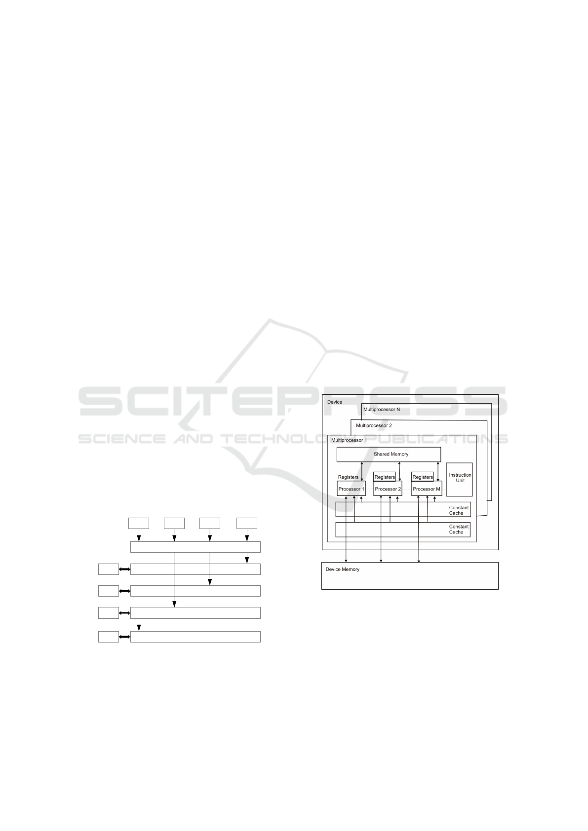
2 GPGPU AND

MULTIPROCESSOR

COMPUTING

The architecture of a GPGPU card is described in

Fig. 2. GPGPU is constructed as N multiproces-

sor structure with M cores each. The cores share an

Instruction Unit with other cores in a multiproces-

sor. Multiprocessors have dedicated memory chips

which are much faster than global memory, shared

for all multiprocessors. These memories are: read-

only constant/texture memory and shared memory.

The GPGPU cards are constructed as massive paral-

lel devices, enabling thousands of parallel threads to

run which are grouped in blocks with shared mem-

ory. A dedicated software architecture CUDA makes

possible programming GPGPU using high-level lan-

guages such as C and C++ (NVIDIA, 2014). CUDA

requires an NVIDIA GPGPU like Fermi, GeForce

8XXX/Tesla/Quadro etc. This technology provides

three key mechanisms to parallelize programs: thread

group hierarchy, shared memories, and barrier syn-

chronization. These mechanisms provide ﬁne-grained

parallelism nested within coarse-grained task paral-

lelism.

Figure 2: GPGPU architecture.

Creating the optimized code is not trivial and thor-

ough knowledge of GPGPUs architecture is neces-

sary to do it effectively. The main aspects to con-

sider are the usage of the memories, efﬁcient division

of code into parallel threads and thread communica-

tions. As it was mentioned earlier, constant/texture,

shared memories and local memories are specially op-

timized regarding the access time, therefore program-

mers should optimally use them to speedup access to

Parallel Implementation of Spatial Pooler in Hierarchical Temporal Memory

347

data on which an algorithm operates. Another im-

portant thing is to optimize synchronization and the

communication of the threads. The synchronization

of the threads between blocks is much slower than in

a block. If it is not necessary it should be avoided, if

necessary, it should be solved by the sequential run-

ning of multiple kernels. Another important aspect is

the fact that recursive function calls are not allowed in

CUDA kernels. Providing stack space for all the ac-

tive threads requires substantial amounts of memory.

Modern processors consist of two or more inde-

pendent central processing units. This architecture

enables multiple CPU instructions (add, move data,

branch etc.) to run at the same time. The cores

are integrated into a single integrated circuit. The

manufacturers AMD and Intel have developed several

multi-core processors (dual-core, quad-core, hexa-

core, octa-core etc.). The cores may or may not share

caches, and they may implement message passing or

shared memory inter-core communication. The sin-

gle cores in multi-core systems may implement archi-

tectures such as vector processing, SIMD, or multi-

threading. These techniques offer another aspect of

parallelization (implicit to high level languages, used

by compilers). The performance gained by the use

of a multi-core processor depends on the algorithms

used and their implementation.

There are lot of programming models and li-

braries of multi-core programming. The most pop-

ular are pthreads, OpenMP, Cilk++, TDD etc. In our

work OpenMP was used (OpenMP, 2010), being a

software platform supporting multi-threaded, shared-

memory parallel processing multi-core architectures

for C, C++ and Fortran languages. By using OpenMP,

the programmer does not need to create the threads

nor assign tasks to each thread. The programmer in-

serts directives to assist the compiler into generating

threads for the parallel processor platform.

3 HIERARCHICAL TEMPORAL

MEMORY

Hierarchical Temporal Memory (HTM) replicates the

structural and algorithmic properties of the neocortex.

It can be regarded as a memory system which is not

programmed and it is trained through exposing them

to data i.e. text. HTM is organized in the hierarchy

which reﬂects the nature of the world and performs

modeling by updating the hierarchy. The structure is

hierarchical in both space and time, which is the key

in natural language modeling since words and sen-

tences come in sequences which describe cause and

effect relationships between the latent objects. HTMs

may be considered similar to Bayesian Networks,

HMM and Recurrent Neural Networks, but they are

different in the way hierarchy, model of neuron and

time is organized (Hawkins and Ahmad, 2011).

At any moment in time, based on current and past

input, an HTM will assign a likelihood that given con-

cepts are present in the examined stream. The HTM’s

output constitutes a set of probabilities for each of the

learned causes. This moment-to-moment distribution

of possible concepts (causes) is denoted as a belief. If

the HTM covers a certain number of concepts it will

have the same number of variables representing those

concepts. Typically HTMs learn about many causes

and create a structure of them which reﬂects their re-

lationships.

Even for human beings, discovering causes is con-

sidered to be a core of perception and creativity, and

people through course of their life learn how to ﬁnd

causes underlying objects in the world. In this sense

HTMs mimic human cognitive abilities and with a

long enough training, proper design and implemen-

tation, they should be able to discover causes humans

can ﬁnd difﬁcult or are unable to detect (Kapuscinski,

2010)(Sherwin and Mavris, 2009).

HTM infers concepts of new stream elements and

the result is a distribution of beliefs across all the

learned causes. If the concept (e.g. one of the cat-

egories occurring in the examined stream) is unam-

biguous, the belief distribution will be peaked other-

wise it will be ﬂat. In HTMs it is possible to disable

learning after training and still do inference.

4 SPATIAL POOLER IN

HIERARCHICAL TEMPORAL

MEMORIES

This paper focuses on spatial pooler parallelization. It

may be summarized in the following steps:

• Starts with an input consisting of a ﬁxed number

of bits which could be sensory data or they could

come from another region lower in the hierarchy,

• assigns a ﬁxed number of columns in the region

this entry. Each column has an associated seg-

ment of dendrites (Hawkins and Ahmad, 2011).

Dendrite segments have potential synapses. Each

synapse has a permanence value,

• determines number of valid synapses connected to

every column,

• boosting factor is used to amplify value of

columns. It is evaluated on the base of a given

column neighbours,

ICAART 2016 - 8th International Conference on Agents and Artiﬁcial Intelligence

348

• the columns which are selected by the boosting

procedure inhibit all the neighbours within the in-

hibition radius,

• all the active columns have their synapses’ per-

manence values adjusted. The ones aligned with

active inputs are increased.

The detailed implementation of the algorithm is as

follows:

• Each column is connected by a ﬁxed number of

inputs to randomly selected node inputs. Based

on the input pattern, some columns will receive

more active input values,

• Inputs of columns (synapses) have values (ﬂoat-

ing point between 0 and 1 called permanence

value) which represents possibility of activating

the synapse (if the value is greater than 0.5 and

corresponding input is 1 the synapse is active),

• Columns which have more active connected

synapses than given threshold (minOverlap) and

its overlap parameter (number of active synapses)

is better than k-th overlap of set of columns in

spectrum of inhibition radius,

• During learning process columns gather informa-

tion about their history of activity, overlap values

(if overlap was greater than minOverlap or not),

compute minimum and maximum overlap duty

cycle and then decides according to the combina-

tions of these parameters if their permanence val-

ues or inhibition radius should be changed.

Generally, spatial pooling selects a relatively con-

stant number of the most active columns and inacti-

vates (inhibits) other columns in the vicinity of the

active ones. Similar input patterns tend to activate a

stable set of columns. The classiﬁer module based

on Spatial Pooler is realized by overlap and activation

computing on incoming input values. The rest of the

parameters are set during learning process. The func-

tionality of Spatial Pooler is similar to LVQ or Self

Organizing Maps neural models.

5 IMPLEMENTATION OF

SPATIAL POOLER IN GPGPU

This section describes GPU implementation of spa-

tial pooler. As mentioned in previous section spe-

cial data structures are needed for spatial algorithm.

Mapping these data structures to GPU memory hi-

erarchy is crucial for effective implementation. The

permanence values, column inputs connections, col-

umn activation, overlapDutyCycle, activeDutyCycle,

minimum and maximum overlapDutyCycle are col-

umn local data structures (see algorithm in section 4).

The overlap, overlapDutyCycle, activeDutyCycle, in-

put data are shared between columns. The representa-

tion of data structures is crucial in efﬁcient algorithm

implementation. Some of the data like activation, val-

ues in overlapDutyCycle and activeDutyCycle arrays

can be represented as a single bit. The representation

width of the rest of the data depends on architecture of

spatial pooler e.g. number of inputs of each column,

ratio between number of columns and input size etc.

The size of representation of data mentioned above

were computed for our simulations as follows:

• overlap, overlap DutyCycle, active DutyCycle

values are stored as array of integers, array size

is equal to blockDim.x · nrOfColumnsPerThread,

• input values for block columns in ar-

ray of size sizeOfInputPerBlock, which

is equal to (2 · radiusO f ColumnInputs ·

blockDim.x · noO fColumnsPerT hread + 2 ·

radiusO fColumnInputs) ÷ 32 (where radiusOf-

ColumnInputs is width of input where single

column can be connected). Dividing by 32 due to

fact that each single input signal is represented by

single bit,

• activation as single bit or byte (depends on con-

ﬁguration),

• overlap window, activation window arrays as in-

teger values with single bits inside representing if

column was overlapped or activated in last 32 pre-

vious cycles,

• minimum DutyCycle, maximum DutyCycle as ar-

rays of ﬂoat values, array size is equal to nrOf-

ColumnsPerThread,

• column connections inputs indexes as byte ar-

rays (size equal to nrOfColumnsPerThread ·

noColInputs), permanence values as ﬂoat arrays

(nrOfColumnsPerThread · noColInputs)

• positions of central indexes column inputs store in

integer arrays of size nrOfColumnsPerThread.

The Tesla M2090 has 48kB of shared memory per

each block and 32kB register memory which can be

divided between block threads. In our work three dif-

ferent conﬁgurations were implemented (each conﬁg-

uration run with 64 threads per block):

• thread processing one column with majority of

local column data (column data not shared be-

tween other columns) stored in registers (minor-

ity in local thread memory), radiusOfColumnIn-

puts is 128, each column has 32 input connec-

tions, where all local column data stored in regis-

ters, shared data in block shared memory, the size

Parallel Implementation of Spatial Pooler in Hierarchical Temporal Memory

349

of data in local thread memory is: (32 + 32 · 4),

the data in registers: 6 · 4 + 1 as six four bytes val-

ues are stored and one byte for activation, the size

of data in shared memory is (3 · 4 · blockDim.x +

sizeO f InputPerBlock), which is equal in our case

(12 · 64 + (2 · 32 ·64 + 2 ·32) ÷ 32) (ﬁgure 3),

• thread processing eight columns with local col-

umn data stored in local memory and registers,

radiusOfColumnInputs is 128, each column has

32 input connections, shared data of size (3 ·

4 · blockDim + sizeO f InputPerBlock) in shared

memory, the size of data in thread local memory

is: 5 · 4 · 8 + 8 · 32 · (1 + 4), the data in registers:

1 + 4, the size of data in shared memory is the

same as in previous conﬁguration (ﬁgure 4),

• thread processing eight columns with shared data

ﬁlled as much as possible, only column inputs in-

dexes, their permanence values are stored in lo-

cal memory, the size of data in local memory is:

8 · 32 · (1 + 4), the data in registers: 1 + 4, the

size of data in shared memory is sum of (3 · 4 ·

blockDim + sizeO f InputPerBlock) and 5 · 4 · 8.

Registers

Local Memory L1/L2

Global Memory

Shared Memory

curand states[]

int inputs[]

int overlapTab[blockDim.x]

int overlapDutyCycle[blockDim.x]

int inputShared[sizeOfInputPerBlock]

int activeDutyCycle[blockDim.x]

byte cInputs[noColInputs]

float pValues[noColInputs]

byte Activation

curandState cState

int overlapWindow

int activationWindow

float minDutyCycle

float maxDutyCycle

int pos

Figure 3: HTM architecture in GPU for 1 column processed

by thread.

Random seed generator is stored always in reg-

isters. The main goal is to parameterized spatial

pooler that as much as possible local column data

ﬁt available registers and local memory for single

Registers

Local Memory L1/L2

Global Memory

Shared Memory

curand states[]

int inputs[]

int overlapTab[blockDim.x*nrOfColumnsPerThread]

int overlapDutyCycle[blockDim.x*nrOfColumnsPerThread]

int inputShared[sizeOfInputPerBlock]

int activeDutyCycle[blockDim.x*nrOfColumnsPerThread]

int overlapWindow[ ]

int activationWindow[

nrOfColumnsPerThread

nrOfColumnsPerThread]

float minDutyCycle[nrOfColumnsPerThread]

float maxDutyCycle[nrOfColumnsPerThread]

byte cInputs[nrOfColumnsPerThread*noColInputs]

float pValues[nrOfColumnsPerThread*noColInputs]

int pos[nrOfColumnsPerThread]

byte Activation

curandState cState

Figure 4: HTM architecture in GPU for 8 columns pro-

cessed by thread.

block thread. The shared data should ﬁt shared block

memory. The shared data should be allocated in

such manner that avoids bank conﬂicts (threads sin-

gle intruction should read or write data from differ-

ent banks). The input data stored in shared mem-

ory is the only one array with random access patterns

and there is no way to avoid bank conﬂicts while its

reading. The input signals represented by bits sig-

niﬁcantly decrease memory requirements. The algo-

rithm in GPGPU ﬁrstly initializes by seperate ker-

nel initialize curand random generator and stores the

seeds in global memory. Then HTM kernel reads in

coalesced manner input values and seed from global

memory and stores them in shared memory and regis-

ters, respectively. After that initializing column pro-

cess is executed (random starting permanence values

and connection indexes are generated and stored in

local memory, ﬁgure 4 and ﬁgure 3). Then whole

learning algorithm is executed (cycles of computing

overlap, activation, permanence values updated, du-

tyCycle functions) on data stored in GPU memories.

The columns processed by boundary threads (ﬁrst

thread and thread with blockDim.x-1 indexes) are pro-

cessed with limited data because of the lack of values

of all columns parameters in spectrum of inhibition

radius (boundary effects due to shared and local mem-

ory parameters storing). In case of statistical algo-

rithm like HTM spatial pooler this effect does not has

negative inﬂuence on algorithm quality. Advantage

ICAART 2016 - 8th International Conference on Agents and Artiﬁcial Intelligence

350

of storing data in shared memory during execution

of whole algorithm is lack of global synchronization

between blocks which in case of GPU is time con-

suming. The global synchronization can be solved by

multi kernel invocation but it needs additional global

store and write operations which signiﬁcantly drops

the efﬁciency. As was mentioned in previous section

the classiﬁer module is realized by just implemented

overlap and activation functions. The input data is

transferred from global memory (sizeOfInputShared

for each block) in each cycle of classifying process.

6 IMPLEMENTATION OF

SPATIAL POOLER IN OPENMP

As was mentioned in section 3, programmer by

inserting openmp directives in appropriate places let

compiler to parallelize the code. The spatial pooler

algorithm can be divided to four main sections: col-

umn overlap computing, column activity checking,

permanence values updates and DutyCycles param-

eter computation (Hawkins and Ahmad, 2011). All

these sections are inside while loop are responsible

for learning cycles processing. The iterations of

while loop are dependent. All sections mentioned

above apart from while loop can be fully parallelized.

Therefore omp parallel for directive was used. After

each section a thread barrier is automatically inserted.

The pseudocode of openmp implementation is as

follows:

while (cycle < nr_cycle) {

#pragma omp parallel for

for (nr = 0; nr < nrOfColums; nr++) {

overlapTab[nr]=overlap(nr)

}

#pragma omp parallel for

for (nr = 0; nr < nrofColumns; nr++) {

activation[nr]=checkActivation(nr)

}

#pragma omp parallel for

for (nr = 0; nr < nrOfColumns; nr++) {

if (activation[nr] == 1)

permValueUpdate(nr)

}

#pragma omp parallel for

for (nr=0; nr < nrOfColumns; nr++) {

activeDutyCycle[nr] = \

computeActiveDutyCycle(nr)

maxDutyCycle = computeMaxDutyCycle()

minDutyCycle = computeMinDutyCycle()

overlapDutyCycle[nr] = \

overlapDutyCycle(nr)

}

cycle++

}

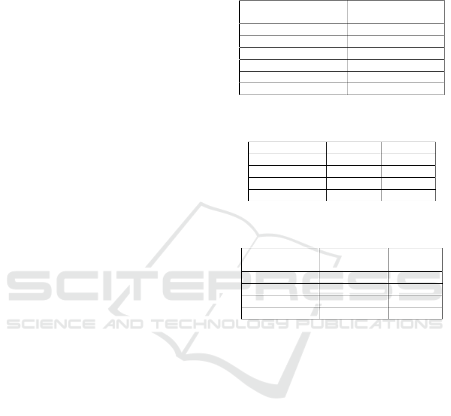
Table 1: Proﬁling of spatial pooler learning algorithm in

CPU.

Method percentage of whole

algorithm execution

column initialization 2.5

overlap 28.4

activation 38.7

permance values update 5

activeDutyCycle 8.5

overlapDutyCycle 9

Table 2: Proﬁling of spatial pooler learning algorithm

in CPU for overlap and activation (noO fColumns ×

noO fColInputs × inhibitationRadius).

Conﬁguration overlap activation

8192 × 32 × 32 28.4 38.7

8192 × 32 × 64 20.5 52.4

4096 × 64 × 32 37 29.6

16384 × 16 × 32 25.9 34.4

Table 3: Proﬁling of spatial pooler learning algo-

rithm in CPU for permanence update and total time

(noO fColumns × noO f ColInputs × inhibitationRadius).

Conﬁguration permanence

update

total time

(ms)

8192 × 32 × 32 5 397

8192 × 32 × 64 2 570

4096 × 64 × 32 5.5 270

16384 × 16 × 32 4.2 593

7 EXPERIMENTAL RESULTS

Tables 1, 2 and 3 present results of proﬁling learn-

ing algorithm of spatial pooler. It is worth noting that

execution time varies signiﬁcantly across code sec-

tions. Activation computing is almost the most com-

putationally exhaustive. However, the proportions

may change for different set-up parameters. This ap-

plies in particular to the overlap computation since it

is the second most computationally demanding sec-

tion. The rest of the functions like minOverlapDu-

tyCycle, maxDutyCycle, boost and inhibitionRadius

update are omitted in tables because their contribu-

tion in whole time is negligible. As proﬁled data and

time of execution of learning algorithm is known it

is possible to estimate efﬁciency of pattern classiﬁer

based on Spatial Pooler (see section 4).

Then experimental tests of learning spatial pooler

algorithm were run. Results were measured with

different parameters. Tables 4 and 5 describe re-

sults gained in Python (1 core CPU, like in NuPic

(Numenta, 2011)), GPU, single and multicore CPU

Parallel Implementation of Spatial Pooler in Hierarchical Temporal Memory

351

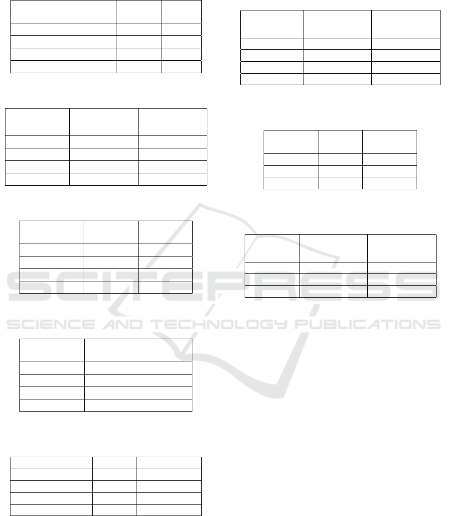
Table 4: Execution times of 100 cycles learning algorithm

in SP on CPU (1 core) and GPU (miliseconds).

Input size

(no.columns)

Python

1 core

GPGPU C/C++

1 core

) 855190 31.4 21019

) 413310 15.0 10250

) 205400 8.4 4100

) 103270 5.5 2590

Table 5: Execution times of 100 cycles learning algorithm

in SP on CPU with vectorized version (miliseconds).

Input size

(no.columns)

CPU (1 core)

(vectorized)

CPU (6 cores)

(vectorized)

) 5160 1419

) 2555 692

) 1255 361

) 613 178

Table 6: Execution times of 100 cycles learning algorithm

in SP in two different GPU conﬁgurations (miliseconds).

Input size

(no.columns)

1 column

per thread

8 columns

per thread

) 154.2 31.4

) 69.9 15.0

) 33 8.4

) 16.32 5.5

Table 7: Execution times of 100 cycles learning algorithm

in SP in full shared memory GPU conﬁguration (milisec-

onds).

Input size

(no.columns)

1 column full shared

memory

) 267.2

) 126.4

) 61.6

) 30.9

Table 8: Execution times of SP for different number of cy-

cles, number of inputs: 524288, number of columns: 8192

(miliseconds).

Number of cycles GPGPU CPU (1 core)

20 2.9 300

40 4.3 555

70 5.7 900

100 6.88 1300

(C implementation). The python implementation is

highly inefﬁcient, more than 50-1000 times slower

than others (from not vectorized CPU to GPU imple-

mentation). The speedups in case of CPU are close

to linear. The GPU implementation is signiﬁcantly

faster than in multicore CPU (up to 40-50 times).

Table 9: Execution times of SP for different number of cy-

cles, number of inputs: 524288, number of columns: 8192

(miliseconds).

Number of

cycles

CPU (1 core)

(vectorized)

CPU (6 cores)

(vectorized)

20 72 24

40 113 41

70 196 69

100 325 100

Table 10: Execution times of SP for different inhibition ra-

dius values, number of inputs: 524288, number of columns:

8192 (miliseconds).

Inhibition

radius

GPGPU CPU

(1 core)

16 6.2 960

32 6.88 1300

64 7.6 2000

Table 11: Execution times of SP for different inhibition ra-

dius values, number of inputs: 524288, number of columns:

8192 (miliseconds).

Inhibition

radius

CPU (1 core)

(vectorized)

CPU (6 cores)

(vectorized)

16 261 66

32 325 100

64 444 147

Tables 6 and 7 depict results in case of three dif-

ferrent GPU spatial pooler conﬁgurations. The last

four tables 8, 9, 10, 11 show times of execution in

case of different number of learning cycles and in-

hibition radius value (the one column processed per

thread version is described in these tables).

Inhibition radius chance has major impact of com-

putations in case of CPU and should be taken into ac-

count when the overall execution time is considered,

Tab. 6. The simulations were run on NIVDIA Tesla

M2090 and Intel Xeon 4565 2.7Ghz. All results pre-

sented in tables are average values collected in ﬁve

measure probes (standard deviation less than 10% of

average values).

8 CONCLUSIONS

Our research shows that high level implementation of

HTM in object languages is highly inefﬁcient. The C

language code run in parallel hardware platform gives

signiﬁcant speedup. It was observed that in case of

vectorized and multicore implementation speed up is

close to linear. The GPGPU outperforms 6-core CPU.

It is worth to say that results measured on CPU with

ICAART 2016 - 8th International Conference on Agents and Artiﬁcial Intelligence

352

more cores should be compared with GPU. Therefore

performance tests of Spatial Pooler on Xeon Phi will

be provided. Our work shows that HTM in hard-

ware accelerators can be used in real-time applica-

tions. Further research, will concentrate on parallel

GPU and multicore Temporal Pooler implementation.

Additionaly, adaption of C source code to OpenCL

should be done to test in other platforms like FPGA

and other heterogenous platforms (Vyas and Zaveri,

2013). At the end comparative studies of efﬁciency

and learning quality should be done among other par-

allel deep learning models.

ACKNOWLEDGEMENTS

This research is supported by the European Regional

Development Program no. POIG.02.03.00-12-137/13

PL-Grid Core.

REFERENCES

Cai, X., Xu, Z., Lai, G., Wu, C., and Lin, X. (2012). Gpu-

accelerated restricted boltzmann machine for collab-

orative ﬁltering. ICA3PP’12 Proceedings of the 12th

international conference on Algorithms and Architec-

tures for Parallel Processing - Volume Part I, pages

303–316.

Cisco (2012). Visual networking index. Visual Networking

Index, Cisco Systems.

Hawkins, J. and Ahmad, S. (2011). Numenta, white pa-

per. Numenta, Hierachical Temporal Memory, white

paper, version 0.2.1, september 12, 2011.

Hilbert, M. and Lopez, P. (2011). The worlds technological

capacity to store, communicate, and compute infor-

mation. In University of Vermont, Vol. 332, no. 6025,

pages 60–65.

Idc (2011). Idc predicts. IDC Predicts 2012 Will Be the

Year of Mobile and Cloud Platform Wars as IT Ven-

dors Vie for Leadership While the Industry Redeﬁnes

Itself. IDC. 2011-12-01.

Kapuscinski, T. (2010). Using hierarchical temporal mem-

ory for vision-based hand shape recognition under

large variations in hands rotation. 10th Interna-

tional Conference, ICAISC 2010, Zakopane, Poland,

in Artiﬁcal Intelligence and Soft Computing, Springer-

Verlag, pages 272–279.

Lopes, N., Ribeiro, B., and Goncalves, J. (2012). Re-

stricted boltzmann machines and deep belief networks

on multi-core processors. Neural Networks (IJCNN),

The 2012 International Joint Conference on, pages 1–

Numenta (2011). Nupic application.

https://github.com/numenta/nupic/wiki.

NVIDIA (2014). Cuda framework.

https://developer.nvidia.com/cuda-gpus.

OpenMP (2010). Openmp library. http://www.openmp.org.

Sherwin, J. and Mavris, D. (2009). Hierarchical tempo-

ral memory algorithms for understanding asymmet-

ric warfare. Aerospace conference, 2009 IEEE, MT,

pages 1–10.

Vyas, P. and Zaveri, M. (2013). Verilog implementation of

a node of hierarchical temporal memory. Asian Jour-

nal of Computer Science and Information Technology,

AJCSIT, 3:103–108.

Wu, X., Zhu, X., Wu, G.-Q., and Ding, W. (2014). Data

mining with big data. Knowledge and Data Engineer-

ing, IEEE Transactions on, 26(1):97–107.

Parallel Implementation of Spatial Pooler in Hierarchical Temporal Memory

353