Fully Automated Image Preprocessing for Feature Extraction from

Knife-edge Scanning Microscopy Image Stacks

Towards a Fully Automated Image Processing Pipeline for Light Microscopic

Images

Shruthi Raghavan and Jaerock Kwon

Department of Electrical and Computer Engineering,

Kettering University, 1700 University Ave., 48504, Flint, MI, U.S.A.

Keywords:

KESM, Artifact Removal, Preprocessing, Tissue Extraction, Image Normalization.

Abstract:

Knife-Edge Scanning Microscopy (KESM) stands out as a fast physical sectioning approach for imaging

tissues at sub-micrometer resolution. To implement high-throughput and high-resolution, KESM images a

tissue ribbon on the knife edge as the sample is being sectioned. This simultaneous sectioning and imaging

approach has following beneﬁts: (1) No image registration is required. (2) No manual job is required for

tissue sectioning, placement or microscope imaging. However spurious pixels are present at the left and right

side of the image, since the ﬁeld of view of the objective is larger than the tissue width. The tissue region

needs to be extracted from these images. Moreover, unwanted artifacts are introduced by KESM’s imaging

mechanism, namely: (1) Vertical stripes caused by unevenly worn knife edge. (2) Horizontal artifacts due

to vibration of the knife while cutting plastic embedded tissue. (3) Uneven intensity within an image due to

knife misalignment. (4) Uneven intensity levels across images due to the variation of cutting speed. This paper

outlines an image processing pipeline for extracting features from KESM images and proposes an algorithm to

extract tissue region from physical sectioning-based light microscope images like KESM data for automating

feature extraction from these data sets.

1 INTRODUCTION

Analysis of biological structures in tissues at sub

micrometer resolution is enabled by techniques like

the Knife Edge Scanning Microscopy (KESM) (May-

erich et al., 2008), Confocal Microscopy (Shot-

ton, 1989), Automatic tape collecting lathe ultra-

microtome (ATLUM) (Hayworth et al., 2006), Se-

rial Block Face Scanning Electron Microscopy (SBF-

SEM) (Denk and Horstmann, 2004) and All Opti-

cal Histology (Tsai et al., 2003). These microscopic

imaging methods are based on either physical or opti-

cal sectioning, or both (ATLUM).

Knife-edge scanning microscopy is the technique

of concurrently slicing and imaging tissue samples at

sub micrometer resolution. This preserves image reg-

istration throughout the depth of the tissue block and

eliminates undesirable events such as back-scattering

of light and bleaching of ﬂuorescent-stained tissue be-

low the knife.

The KESM based high-throughput and high-

resolution tissue scanner has produced multiple

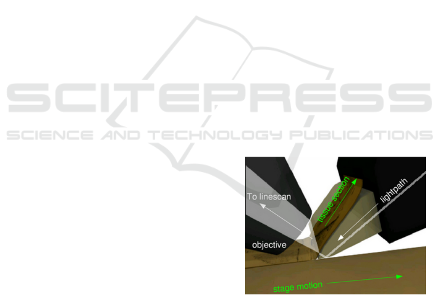
Figure 1: Imaging principles of the KESM.The objective

and the knife is held in place, while the specimen afﬁxed on

the positioning stage moves at the resolution of 20 nm and

travel speed of 1-5, and gets scraped against the diamond

knife (5 mm wide for 10X objective), generating a thin sec-

tion ﬂowing over the knife. Imaging happens at knife-edge.

Direction of movement of light and stage is indicated with

solid arrows. (Adopted from (Choe et al., 2011)).

datasets till date. A diamond knife is used as colli-

mator and also to section the tissue as illustrated in

Raghavan, S. and Kwon, J.

Fully Automated Image Preprocessing for Feature Extraction from Knife-edge Scanning Microscopy Image Stacks - Towards a Fully Automated Image Processing Pipeline for Light Microscopic

Images.

DOI: 10.5220/0005708700930100

In Proceedings of the 9th International Joint Conference on Biomedical Engineering Systems and Technologies (BIOSTEC 2016) - Volume 2: BIOIMAGING, pages 93-100

ISBN: 978-989-758-170-0

Figure 1. The tissue sample being sliced by the knife

is imaged just above the knife edge by a powerful line

scan camera. The image capture mechanism is trig-

gered based on the encoded position of the tissue be-

ing sliced, which ensures that every sectioning results

in an image capture. The KESM can image a 1cm

tissue block in approximately 50 hours at a resolution

of 0.6µm × 0.7µm × 1.0µm.

To get information from this data, the KESM im-

ages have to be preprocessed followed by feature ex-

traction and post-processing if necessary. This pa-

per describes the ﬁrst preprocessing step in an image

processing pipe that is being designed for automat-

ing feature extraction and sharing. A novel method

for extraction of tissue regions is being proposed for

physical sectioning-based light-microscope imaging

data.

2 BACKGROUND

While sectioning and imaging in KESM, width of the

tissue slice is not exactly the ﬁeld of view of the ob-

jective. Thus, there is additional non-tissue area that

appears as dark regions on either side of the tissue

in every image. The additional region causes signif-

icant increase in the amount of memory required by

applications that process the images. For instance, as-

sume we imaged a tissue sample using KESM. Let the

width of a line scan image be 4096 pixels and a slice

consist of 12000 lines. If pixels are a byte each, the

raw KESM image will occupy 46.875MB. However,

if tissue width is only 2400pixels, only 27.466MB of

memory is actually useful. KESM could collect ter-

abytes of images and 41.41% reduction in image size

will signiﬁcantly improve the efﬁciency of feature ex-

traction.

Ideally, the tissue region should be at a ﬁxed lo-

cation in the image. This would make it possible to

crop all images in a given column at the same posi-

tion, given the tissue width. However, this is not al-

ways the case. In case of interruptions in the imaging

process like power outages and clogging in the wa-

ter circulation, the KESM might need to be stopped

for maintenance and the setup might be disturbed. In

such scenarios, after restarting the KESM, the start

of tissue may not be at the same pixel position in the

image as before. In this case, cropping at ﬁxed posi-

tion may cause loss of tissue data. This necessitates

detection of the tissue edge for every image.

Each tissue sample imaged by the KESM can gen-

erate up to around 80,000 images (the tissue is lat-

erally sectioned several times and each column has

around 10,000 images). Thus, to extract tissue region

manually requires a lot of time and effort and is inefﬁ-

cient. So we need image processing to automate this.

A template matching based method was proposed for

tissue extraction from the KESM image stacks (Kwon

et al., 2011). However, this method suffered from a

high error rate. The novel algorithm for tissue extrac-

tion proposed in this paper has lower error rates and

is more efﬁcient in automation of the process.

Knife chatter and illumination artifacts affect

KESM images as shown in Figure 9. Varying cut-

ting speeds introduced to reduce knife chatter cause

inter-image intensity differences. These artifacts hin-

der visualization and feature extraction. So inter- and

intra- image normalization is also a necessary prepro-

cessing step for KESM stacks.

3 METHOD

This section explains the newly proposed tissue area

detection and extraction algorithm. It focuses on the

reasoning behind the methodology used. We also de-

scribe the method used for intensity normalization al-

gorithm as proposed in (Kwon et al., 2011) for com-

pleteness.

3.1 Tissue Area Detection

The image from the KESM consists of a right and a

left edge of tissue as shown in Figure 2(a). Figure

2(b) shows the seemingly sharp right-edge. However,

Figure 2(c) reveals gradual decay in the intensity pro-

ﬁle of the right edge. Moreover, KESM is affected

by multiple artifacts as described earlier. For this rea-

son, we do not use the Sobel (Duda et al., 1973), Pre-

witt (Prewitt, 1970) and similar edge detectors. The

Canny edge detector (Canny, 1986) is robust to noise

(Maini and Aggarwal, 2009) but is complex to com-

pute and gives us additional information about cor-

ners that we do not need. Hence, we take the Gaussian

gradient, which can smooth the image before detect-

ing edge gradients to give us a clear right edge loca-

tion. The Gaussian Gradient applies a ﬁlter in the x

and y directions of the two dimensional tissue image

being processed. The equations for ﬁrst order Gaus-

sian derivatives of Gaussian are as given below:

dG(x, y, σ)

−x

2πσ

−(x

)

2σ

(1)

dG(x, y, σ)

−y

2πσ

−(x

)

2σ

(2)

,where x and y represent the kernel location starting

with zeros at the center and σ represents the standard

BIOIMAGING 2016 - 3rd International Conference on Bioimaging

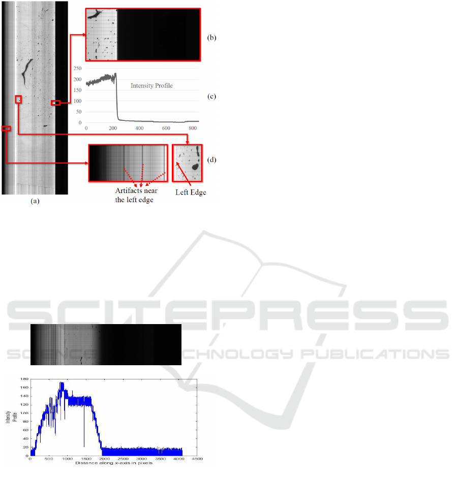
Figure 2: Showing the spurious data and edges of tissue re-

gion in image. (a) One Tissue Slice from KESM microvas-

culature data stack. (b) Right Edge of Tissue expanded

shows sharp demarcation. (c) Intensity Proﬁle along x axis

(distance in pixels from the left side of the image shown

in (b)) shows a gradual gradient that might cause spurious

edge detection by some edge operators. (d) Left edge (the

solid arrow) of tissue expanded shows vertical noise lines

(dotted arrows) that have to be distinguished from the real

left edge.

(a)

(b)

Figure 3: A horizontal section from a KESM image with

no clear right edge necessitating left edge detection. (a)

A small horizontal section of KESM image with occluded

right edge. (b) Intensity proﬁle along the x axis of the image

shown in (a)

deviation of the Gaussian distribution. Smoothing ef-

fect of the Gaussian Kernel, increases as σ increases.

This algorithm does not work with right-occluded

images. Figure 3 shows a horizontal section from a

KESM image with no clear right edge. It is seen that

the edge like proﬁle occurs much before the actual

image edge. In these cases we try to detect the left

edge of tissue to crop the image. It is challenging due

to vertical noise artifacts produced by illumination ir-

regularities in the KESM shown in Figure 2(d).

The technique used to ﬁnd the left edge relies on

the fact that in KESM images, only the correct left

edge has more horizontal as well as vertical gradients.

To use this information efﬁciently, we ﬁrst take the

horizontal followed by the vertical Gaussian gradient

of the image. This leaves us with a strong response at

the left edge. We then use a thresholding to eliminate

the weak responses of vertical noise outside the left

tissue edge. Then, the image is optionally eroded with

a slightly elongated rectangular structuring element to

strengthen edges that remain.

To detect the position of the strong vertical re-

sponse from this image, we use probabilistic hough

line (Galamhos et al., 1999) estimation with one sin-

gle angle (zero) and a decreasing line length starting

from half the height of the entire image. The location

of the longest vertical line found in the left half of the

image is taken to be the index of the left edge.

Rarely, a KESM image is so dark that neither the

left edge nor the right edge of the tissue can be reli-

ably found by the proposed algorithm. Our effort to

make the image processing pipeline fully automated

involved using a best-effort thresholding based tis-

sue region detection algorithm. Minimum cross en-

tropy approach has proven to be a useful segmenta-

tion method in many applications and it has been used

in (Yi-de et al., 2004; Sarkar et al., 2011; Al-Attas

and El-Zaart, 2007) efﬁciently, which is empirical ev-

idence for effectiveness of this threshold. So in our

algorithm, we used Li threshold (Li and Lee, 1993)

that is based this thresholding. Thus the proposed au-

tomated algorithm will extract the tissue region from

every single image generated by the KESM, with

best-effort cropping for very occluded or dark images.

3.2 Image Intensity Normalization

We implemented the image intensity equalization al-

gorithm previously proposed for KESM image stacks

(Kwon et al., 2011). Brieﬂy, this method normalizes

each pixel in a row or column based on the median

intensity value of that row or column. This procedure

is applied to all rows and columns in the image to

achieve uniform intensity. We also adopt the method

of selective normalization and set a threshold for fore-

ground segmentation when the median intensity is too

low to get a clear distinction between tissue and back-

ground. It alleviates artifacts and translates all images

to a common background intensity level.

Fully Automated Image Preprocessing for Feature Extraction from Knife-edge Scanning Microscopy Image Stacks - Towards a Fully

Automated Image Processing Pipeline for Light Microscopic Images

4 IMPLEMENTATION

The algorithm for tissue extraction developed in this

paper consists of three logical divisions - edge detec-

tion, admissibility check and cropping. Edge is de-

tected using one of the two methods explained below

or by thresholding based right edge detection. The

overview of the algorithm ﬂow is shown in Figure 4.

Once the tissue region is extracted from the image,

a normalization algorithm is applied to enable further

processing. The interested reader is referred to (Kwon

et al., 2011) for the implementation details.

Right

Edge

Detection

Admissible

Right Edge?

Left

Edge

Detection

Best Effort

Min. Cross

Entropy

Threshold

Admissible

Left Edge?

Extract

Tissue

Region

YES

Input

Figure 4: Flowchart showing the logical structure of pro-

posed automated cropping algorithm

4.1 Right Edge Detection for Tissue

Extraction

The right edge detection algorithm involves ﬁnding

the right edge at the strongest Gaussian gradient re-

Algorithm 1: Right Edge Detection.

1: function FIND RIGHT EDGE

2: init

3: image ← image ∗

dG(x,y,2)

4: image ← image ∗

dG(x,y,2)

5: y,x ← Non-zero Indices from image

6: xo ← (val,occ) in x,sorted by freq. of val

7: x ← xo for 10 highest ”val” in xo

8: index ← val with max(occ) x

9: return index

sponse on the right half of image. The Gaussian gradi-

ent function with sigma of 2 is applied. First, the hor-

izontal derivative of Gaussian is convolved with the

image (convolution is indicated by ∗) and then the re-

sult is convolved with vertical derivative of Gaussian.

Ideally, this gives an image with its last non-zero pixel

along the x-axis at the right edge of tissue in the im-

age. However, to ensure the algorithm is picking the

most well deﬁned edge, the largest non-zero x-index

(val) that corresponds most occurrences (occ) of non-

zero pixels in y is chosen as the result. The pseudo-

code for this procedure is given in Algorithm 1. This

works for any KESM image that has sufﬁcient con-

trast at the right edge. However, if the right edge of

tissue is too dark or blurred to recover due to artifacts

introduced by the imaging mechanism, this will not

give the correct right edge location. The result pro-

vided by this right edge detection function is validated

by an admissibility test based on tissue width (Tis-

sueWidth), sanity checks and image properties near

detected edge. If the result is admissible, it is used

to crop the tissue from [index-TissueWidth,index]. If

not, the left edge detection algorithm, described next,

is used to try and ﬁnd the index of the left edge of

tissue region.

4.2 Left Edge Detection for Tissue

Extraction

The left edge detection algorithm works by isolat-

ing the edge with greater vertical connectivity and

also maximum horizontal gradients on the left half of

the image. The Gaussian gradient works with lesser

smoothing than for right edge detection. This is to

ensure we do not smooth out the gradient information

we are trying to detect on the left edge. After this edge

Algorithm 2: Left Edge Detection.

1: function FIND LEFT EDGE

2: init

3: image ← image ∗

dG(x,y,1)

4: image ← image ∗

dG(x,y,1)

5: image ← Triangle thresholded image

6: image ← BinaryErode(image)

7: roi lines ← WIDTH - TissueWidth

8: image ← image[0:roi lines]

9: while lines == [ ] and height 6= 0 do

10: lines ← hough lines(image,height)

11: height ← height - predeﬁned dec step

12: if lines == [ ] then

13: return fail

14: index ← x inx of longest line found

15: return index

BIOIMAGING 2016 - 3rd International Conference on Bioimaging

detection step, we apply a triangle threshold to bina-

rize the image. This image is then given as an input to

a binary erode ﬁlter using a narrow rectangular struc-

turing element. This ensures that only the strongest

vertical lines survive. Then probabilistic hough lines

are found in the y-direction and the highest connected

vertical line which in turn is the tallest line found is

taken as being at the position of the left edge. The

x-index at which this line was found is returned to the

cropping algorithm. The pseudo-code for this proce-

dure is given in Algorithm 2.

If the left edge found is admissible, tissue region

is extracted with the result index value. If not, the

image is cropped with a best effort algorithm based on

minimum cross entropy threshold (Li and Lee, 1993).

The image is ﬁrst thresholded based on this method.

Then the strongest vertical edge in the image that is

farthest to the right is taken as the right edge of the

tissue region.

5 VALIDATION

Validation with a real data subset is impractical be-

cause we have to manually ﬁnd the correct tissue

edge in each image. This would be subjective, er-

ror prone and cannot be considered ground truth. So

the proposed algorithm was validated using synthetic

images. The algorithm was run on a computer with

an AMD-64 quad-core processor running at 3.8GHz

with 8GB RAM.

5.1 Testing Proposed Algorithm

The tissue extraction code itself that was explained

in the implementation section was written in Python.

The code for normalization of the data was written in

C++. Synthetic images were generated using a python

script. They mimic the properties of KESM images

and their artifacts. They faithfully reproduce the na-

ture of the edges of tissues in KESM data. An exam-

ple of an image generated by this algorithm is shown

in Figure 5(a). The edge properties are shown in Fig-

ure 5(b) and (c). Thus, we can assume that the results

from the synthetic data are directly representative of

those from KESM data. We tested the proposed crop-

ping algorithm on hundred synthetic images. From

this, the average and maximum errors were found to

be 2.68 pixels and 7 pixels respectively.

(a)

(b)

(c)

Left Edge

Artifacts near the left edge

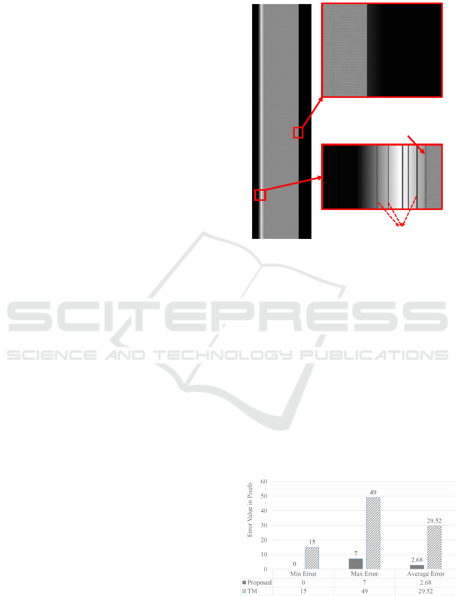
Figure 5: Synthetic image. It has edge properties that mimic

the real KESM images. These images can thus serve as

ground truth for validation of results from the proposed al-

gorithm. (a) Full synthetic image. (b) Right edge magniﬁed.

5.2 Comparitive Evaluation

We also compared the proposed method to a previ-

ously proposed algorithm for tissue extraction. The

algorithm being compared is the template match-

ing(TM) based cropping algorithm proposed in

(Kwon et al., 2011). Error in the number of pix-

els for both these methods is compared in the chart

shown in Figure 6. From this we infer that the pro-

posed algorithm has improved error rate by 90.92%

compared to the template matching based algorithm.

The minimum error for the template matching based

algorithm for the same set of synthetic images is 15

pixels whereas the proposed algorithm is capable of

Figure 6: Quantitative comparison between the proposed

algorithm for tissue extraction and the template matching

algorithm from (Kwon et al., 2011).

Fully Automated Image Preprocessing for Feature Extraction from Knife-edge Scanning Microscopy Image Stacks - Towards a Fully

Automated Image Processing Pipeline for Light Microscopic Images

cropping images with zero error. Figure 7 shows the

result of cropping using the two methods on a syn-

thetic image. Clearly, the proposed algorithm has bet-

ter accuracy in locating the edge of tissue region in

the image.

Error Pixels

(a)

(b)

(c)

(d)

Figure 7: Comparison of cropping using proposed method

and template matching method on a synthetic image for

qualitative results. (a) A small horizontal portion from a

synthetic image. Right edge location = 3442(x). (b) Output

of template matching algorithm proposed in (Kwon et al.,

2011). (c) Output of proposed algorithm cropped at 3442(x)

with zero error. (d) Magniﬁed result from the rectangle

shown in (b) indicating erroneous pixels near the right edge

after cropping, crop location = 3459(x).

6 REPRESENTATIVE RESULTS

We ran the proposed cropping algorithm on the mouse

brain vasculature data stacks imaged by the KESM.

We could crop the entire image stack and also nor-

malize all the images after cropping. This method was

robust enough to work on very dark, very bright and

images affected by different artifacts that are common

in KESM including illumination artifacts. This can be

seen in Figure 9. Each of the ﬁgures show the orig-

inal, cropped and normalized versions of the KESM

images that have been affected by different artifacts.

The traced result shown in Figure 8 was gener-

ated using the All Path Pruning 2.0 (APP2) (Xiao and

Peng, 2013) plug-in in Vaa3D (Peng et al., 2010). De-

fault APP2 parameters were used for the trace except

the background threshold that was set to −1. The

KESM image stack was inverted to have a bright fore-

ground tissue area on a dark background.

7 CONCLUSION AND FUTURE

WORK

A new algorithm has been proposed to extract tis-

sue region from physical sectioning based light mi-

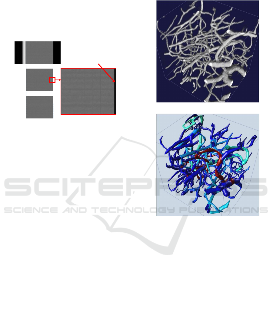
(a)

(b)

Figure 8: 3D visualization of the image data. (a) 3D view

of a properly cropped image volume using the proposed al-

gorithm. The dimension of the image is 153 × 179 × 177

scaled by 0.6 × 0.7 × 1.0 ratio (b) A blood vessel trace re-

sult of (a) using the Vaa3D (Peng et al., 2010) plugin based

on the All Path Pruning 2.0 (APP2) algorithm (Xiao and

Peng, 2013).

croscopy image stacks. The algorithm was developed

using the mouse brain vasculature data set generated

by the KESM. The challenges were mainly the vary-

ing nature of KESM images, which the algorithm was

designed to handle. This made it possible to crop

the entire image stack automatically with high ac-

curacy. The average error for the proposed method

was found to be less than 3 pixels from tests on syn-

thetic data. This was compared against a previously

proposed method for tissue extraction and quantita-

tive comparison results have been shown in the paper.

This algorithm along with normalization, is part of

preprocessing.

An image processing pipeline of our design is pro-

posed as shown in Figure 10. The goal is to automat-

BIOIMAGING 2016 - 3rd International Conference on Bioimaging

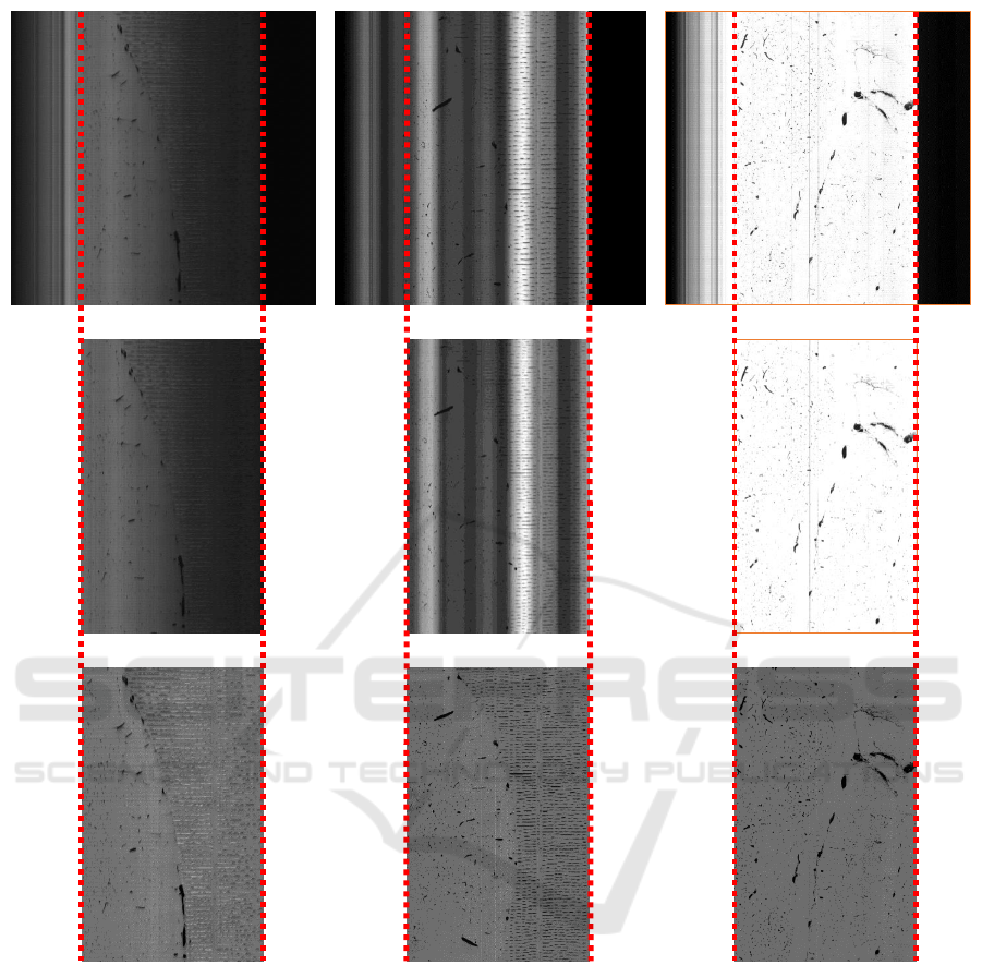
(a) (b) (c)

Figure 9: Results of proposed algorithm to ﬁnd tissue edge under different conditions and the output of normalization algo-

rithm. A small portion from a sample KESM image (top row). The image cropped using proposed tissue extraction algorithm

(middle row). Image normalized using algorithm adapted from (Kwon et al., 2011) (bottom row). (a) A very dark KESM

image (brightness increased for viewing only), the extracted tissue region and its normalized version. (b) A KESM image

with severe illumination artifacts in the form of vertical bands that could be mistaken for edges, the extracted tissue region

and its normalized version. (c) A very bright KESM image, the extracted tissue region and its normalized version.

ically extract the important biological features from

light microscopy images and also publish it online for

the scientiﬁc community to access.

ACKNOWLEDGEMENTS

This material is based upon work supported by the

National Science Foundation (NSF) #1337983.

Fully Automated Image Preprocessing for Feature Extraction from Knife-edge Scanning Microscopy Image Stacks - Towards a Fully

Automated Image Processing Pipeline for Light Microscopic Images

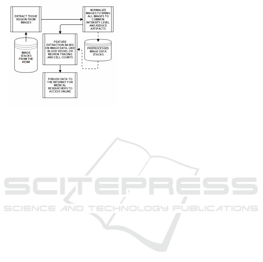
Figure 10: A pipeline to be implemented for information

extraction from the KESM and other physical sectioning-

based microscope image stacks

REFERENCES

Al-Attas, R. and El-Zaart, A. (2007). Thresholding of med-

ical images using minimum cross entropy. In 3rd

Kuala Lumpur International Conference on Biomed-

ical Engineering 2006, pages 296–299. Springer.

Canny, J. (1986). A computational approach to edge detec-

tion. Pattern Analysis and Machine Intelligence, IEEE

Transactions on, (6):679–698.

Choe, Y., Mayerich, D., Kwon, J., Miller, D. E., Sung,

C., Chung, J. R., Huffman, T., Keyser, J., and Ab-

bott, L. C. (2011). Specimen preparation, imaging,

and analysis protocols for knife-edge scanning mi-

croscopy. (58):e3248.

Denk, W. and Horstmann, H. (2004). Serial block-

face scanning electron microscopy to reconstruct

three-dimensional tissue nanostructure. PLoS Biol,

2(11):e329.

Duda, R. O., Hart, P. E., et al. (1973). Pattern classiﬁcation

and scene analysis. J. Wiley and Sons.

Galamhos, C., Matas, J., and Kittler, J. (1999). Progres-

sive probabilistic hough transform for line detection.

In Computer Vision and Pattern Recognition, 1999.

IEEE Computer Society Conference on., volume 1.

IEEE.

Hayworth, K., Kasthuri, N., Schalek, R., and Lichtman, J.

(2006). Automating the collection of ultrathin serial

sections for large volume tem reconstructions. Mi-

croscopy and Microanalysis, 12(S02):86–87.

Kwon, J., Mayerich, D., and Choe, Y. (2011). Automated

cropping and artifact removal for knife-edge scanning

microscopy. In Biomedical Imaging: From Nano

to Macro, 2011 IEEE International Symposium on,

pages 1366–1369. IEEE.

Li, C. H. and Lee, C. (1993). Minimum cross entropy

thresholding. Pattern Recognition, 26(4):617–625.

Maini, R. and Aggarwal, H. (2009). Study and comparison

of various image edge detection techniques. Interna-

tional journal of image processing (IJIP), 3(1):1–11.

Mayerich, D., Abbott, L., and McCormick, B. (2008).

Knife-edge scanning microscopy for imaging and re-

construction of three-dimensional anatomical struc-

tures of the mouse brain. Journal of microscopy,

231(1):134–143.

Peng, H., Ruan, Z., Long, F., Simpson, J. H., and Myers,

E. W. (2010). V3d enables real-time 3d visualization

and quantitative analysis of large-scale biological im-

age data sets. Nature biotechnology, 28(4):348–353.

Prewitt, J. M. (1970). Object enhancement and extraction.

Picture processing and Psychopictorics, 10(1):15–19.

Sarkar, S., Patra, G. R., and Das, S. (2011). A differ-

ential evolution based approach for multilevel image

segmentation using minimum cross entropy threshold-

ing. In Swarm, Evolutionary, and Memetic Comput-

ing, pages 51–58. Springer.

Shotton, D. M. (1989). Confocal scanning optical mi-

croscopy and its applications for biological speci-

mens. Journal of Cell Science, 94(2):175–206.

Tsai, P. S., Friedman, B., Ifarraguerri, A. I., Thompson,

B. D., Lev-Ram, V., Schaffer, C. B., Xiong, Q., Tsien,

R. Y., Squier, J. A., and Kleinfeld, D. (2003). All-

optical histology using ultrashort laser pulses. Neuron,

39(1):27–41.

Xiao, H. and Peng, H. (2013). App2: automatic tracing of

3d neuron morphology based on hierarchical pruning

of a gray-weighted image distance-tree. Bioinformat-

ics, 29(11):1448–1454.

Yi-de, M., Qing, L., and Zhi-Bai, Q. (2004). Automated im-

age segmentation using improved pcnn model based

on cross-entropy. In Intelligent Multimedia, Video and

Speech Processing, 2004. Proceedings of 2004 Inter-

national Symposium on, pages 743–746. IEEE.

BIOIMAGING 2016 - 3rd International Conference on Bioimaging

100