
Domain Specific Author Attribution based on Feedforward Neural
Network Language Models
Zhenhao Ge and Yufang Sun
School of Electrical and Computer Engineering, Purdue University, West Lafayette, Indiana, U.S.A.
Keywords:
Authorship Attribution, Neural Networks, Language Modeling.
Abstract:
Authorship attribution refers to the task of automatically determining the author based on a given sample of
text. It is a problem with a long history and has a wide range of application. Building author profiles using
language models is one of the most successful methods to automate this task. New language modeling methods
based on neural networks alleviate the curse of dimensionality and usually outperform conventional N-gram
methods. However, there have not been much research applying them to authorship attribution. In this paper,
we present a novel setup of a Neural Network Language Model (NNLM) and apply it to a database of text
samples from different authors. We investigate how the NNLM performs on a task with moderate author set
size and relatively limited training and test data, and how the topics of the text samples affect the accuracy.
NNLM achieves nearly 2.5% reduction in perplexity, a measurement of fitness of a trained language model
to the test data. Given 5 random test sentences, it also increases the author classification accuracy by 3.43%
on average, compared with the N-gram methods using SRILM tools. An open source implementation of our
methodology is freely available at https://github.com/zge/authorship-attribution/.
1 INTRODUCTION
Authorship attribution refers to the task of identifying
the text author from a given text sample, by finding
the author’s unique textual features. It is possible to
do this because the author’s profile or style embodies
many characteristics, including personality, cultural
and educational background, language origin, life ex-
perience and knowledge basis, etc. Every person has
his/her own style, and sometimes the author’s iden-
tity can be easily recognized. However, most often
identifying the author is challenging, because author’s
style can vary significantly by topics, mood, environ-
ment and experience. Seeking consistency or consis-
tent evolution out of variation is not always an easy
task.
There has been much research in this area. Juola
(Juola, 2006) and Stamatatos (Stamatatos, 2009) for
example, have surveyed the state of the art and pro-
posed a set of recommendations to move forward.
As more text data become available from the Web
and computational linguistic models using statistical
methods mature, more opportunities and challenges
arise in this area (Koppel et al., 2009). Many statisti-
cal models have been successfully applied in this area,
such as Latent Dirichlet Allocation (LDA) for topic
modeling and dimension reduction (Seroussi et al.,
2011), Naive Bayes for text classification (Coyotl-
Morales et al., 2006), Multiple Discriminant Analysis
(MDA) and Support Vector Machines (SVM) for fea-
ture selection and classification (Ebrahimpour et al.,
2013). Methods based on language modeling are also
among the most popular methods for authorship attri-
bution (Ke
ˇ
selj et al., 2003).
Neural networks with deep learning have been
successfully applied in many applications, such as
speech recognition (Hinton et al., 2012), object detec-
tion (Krizhevsky et al., 2012), natural language pro-
cessing (Socher et al., 2011), and other pattern recog-
nition and classification tasks (Bishop, 1995), (Ge and
Sun, 2015). Neural Network based Language Mod-
els (NNLM) have surpassed the performance of tradi-
tional N-gram LMs (Bengio et al., 2003), (Mnih and
Hinton, 2007) and are purported to generalize better
in smaller datasets (Mnih, 2010). In this paper, we
propose a similar NNLM setup for authorship attri-
bution. The performance of the proposed method de-
pends highly on the settings of the experiment, in par-
ticular the experimental design, author set size and
data size (Luyckx, 2011). In this work, we focused
on small datasets within one specific text domain,
where the sizes of the training and test datasets for
each author are limited. This often leads to context-
Ge, Z. and Sun, Y.
Domain Specific Author Attribution based on Feedforward Neural Network Language Models.
DOI: 10.5220/0005710005970604
In Proceedings of the 5th International Conference on Pattern Recognition Applications and Methods (ICPRAM 2016), pages 597-604
ISBN: 978-989-758-173-1
Copyright
c
2016 by SCITEPRESS – Science and Technology Publications, Lda. All rights reserved
597
biased models, where the accuracy of author detection
is highly dependent on the degree to which the topics
in training and test sets match each other (Luyckx and
Daelemans, 2008). The experiments we conceive are
based on a closed dataset, i.e. each test author also
appears in the training set, so the task is simplified to
author classification rather than detection.
The paper is organized as follows. Sec. 2 intro-
duces the database used for this project. Sec. 3 ex-
plains the methodology of the NNLM, including cost
function definition, forward-backward propagation,
and weight and bias updates. Sec. 4 describes the
implementation of the NNLM, provides the classifica-
tion metrics, and compares results with conventional
baseline N-gram models. Finally, Sec. 5 presents the
conclusion and suggests future work.
2 DATA PREPARATION
The database is a selection of course transcripts from
Coursera, one of the largest Massive Open Online
Course (MOOC) platforms. To ensure the author de-
tection less replying on the domain information, 16
courses were selected from one specific text domain
of the technical science and engineering fields, cov-
ering 8 areas: Algorithm, Data Mining, Information
Technologies (IT), Machine Learning, Mathematics,
Natural Language Processing (NLP), Programming
and Digital Signal Processing (DSP). Table 1 lists
more details for each course in the database, such as
the number of sentences and words, the number of
words per sentence, and vocabulary sizes in multiple
stages. For privacy reason, the exact course titles and
instructor (author) names are concealed. However, for
the purpose of detecting the authors, it is necessary to
point out that all courses are taught by different in-
structors, except for the courses with IDs 7 and 16.
This was done intentionally to allow us to investigate
how the topic variation affects performance.
The transcripts for each course were originally
collected in short phrases with various lengths, shown
one at a time at the bottom of the video lectures. They
were first concatenated and then segmented into sen-
tences, using straight-forward boundary determina-
tion by punctuations. The sentence-wise datasets are
then stemmed using the Porter Stemming algorithm
(Porter, 1980). To further control the vocabulary size,
words occurring only once in the entire course or
with frequency less than 1/100, 000 are considered
to have negligible influence on the outcome and are
pruned by mapping them to an Out-Of-Vocabulary
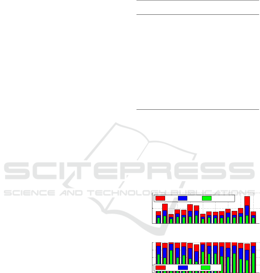
(OOV) mark hunki. The first top bar graph in Fig-
ure 1 shows how the vocabulary size of each course
Table 1: Subtitle database from selected Coursera courses.
ID Field
No. of No. of Words / Vocab. size (original
sentences words sentences / stemmed / pruned)
1 Algorithm 5,672 121,675 21.45 3,972 / 2,702 / 1,809
2 Algorithm 14,902 294055 20.87 6,431 / 4,222 / 2,378
3 DSP 8,126 129,665 15.96 3,815 / 2,699 / 1,869
4 Data Mining 7,392 129,552 17.53 4,531 / 3,140 / 2,141
5 Data Mining 6,906 129,068 18.69 3,008 / 2,041 / 1,475
6 DSP 20,271 360,508 17.78 8,878 / 5,820 / 2,687
7 IT 9,103 164,812 18.11 4,369 / 2,749 / 1,979
8 Mathematics 5,736 101,012 17.61 3,095 / 2,148 / 1,500
9 Machine Learning 11,090 224,504 20.24 6,293 / 4,071 / 2,259
10 Programming 8,185 160,390 19.60 4,045 / 2,771 / 1,898
11 NLP 7,095 111,154 15.67 3,691 / 2,572 / 1,789
12 NLP 4,395 100,408 22.85 3,973 / 2,605 / 1,789
13 NLP 4,382 96,948 22.12 4,730 / 3,467 / 2,071
14 Machine Learning 6,174 116,344 18.84 5,844 / 4,127 / 2,686
15 Mathematics 5,895 152,100 25.80 3,933 / 2,697 / 1,918
16 Programming 6,400 136,549 21.34 4,997 / 3,322 / 2,243
dataset shrinks after stemming and pruning. There are
only 0.5 ∼ 1.5% words among all datasets mapped
to hunki, however, the vocabulary sizes are signifi-
cantly reduced to an average of 2000. The bottom bar
graph provides a profile of each instructor in terms
of word frequency, i.e. the database coverage of the
most frequent k words after stemming and pruning,
where k = 500, 1000,2000. For example, the most
frequent 500 words cover at least 85% of the words in
all datasets.
0 2 4 6 8 10 12 14 16
0
5000
10000
Dataset index (C)
Vocabulary size (V)
Vocabulary size for each dataset
V
original
V
stemmed
V
stemmed−pruned
0 2 4 6 8 10 12 14 16
0.8
0.85
0.9
0.95
1
Dataset index (C)
Database Coverage (DC)
Database coverage from most frequent k words for each dataset
stemmed & pruned datasets, k = 500, 1000, 2000
DC
2000
DC
1000
DC
500
Figure 1: Database profile with respect to vocabulary size
and word coverage in various stages.
3 NEURAL NETWORK
LANGUAGE MODEL
The language model is trained using a feed-forward
neural network illustrated in Figure 2. Given a se-
quence of N words W
1
,W
2
,. ..,W
i
,. .. ,W
N
from
ICPRAM 2016 - International Conference on Pattern Recognition Applications and Methods
598

training text, the network trains weights to predict the
word W
t
, t ∈ [1,N] in a designated target word posi-
tion in sequence, using the information provided from
the rest of words, as it is formulated in Eq. (1).
W
∗
= argmax
t
P(W
t
|W
1
W
2
·· ·W
i
·· ·W
N
), i 6= t (1)
It is similar to the classic N-gram language model,
where the primary task is to predict the next word
given N − 1 previous words. However, here the net-
work can be trained to predict the target word in any
position, given the neighboring words.
IndexofContext
Word
IndexofContext
Word
IndexofContext
Word1
IndexofContext
Word2
⋯⋯
HiddenLayer(sigmoid)
OutputLayer(Softmax)
EmbeddingLayer
Representation
ofWord
Representation
ofWord
Representation
ofWord1
Representation
ofWord2
⋯⋯
IndexofTarget Word
, ∈ 1, ,
Figure 2: Architecture of the Neural Network Language
Model (I: index, W : word, N: number of context words,
W : weight, b: bias).
The network contains 4 different types of layers:
the word layer, the embedding layer, the hidden layer,
and the output (softmax) layer. The weights between
adjacent layers, i.e. word-to-embedding weights
W
word−emb
, embedding-to-hidden weights W
emb−hid
,
and hidden-to-output weights W
hid−out
, need to be
trained in order to transform the input words to the
predicted output word. The following 3 sub-sections
briefly introduce the NNLM training procedure, first
defining the cost function to be minimized, then de-
scribing the forward and backward weight and bias
propagation. The implementation details regarding
parameter settings and tuning are discussed in Sec.
4.
3.1 Cost Function
Given vocabulary size V , it is a multinomial classifi-
cation problem to predict a single word out of V op-
tions. So the cost function to be minimized can be
formulated as
C = −
∑
V
t
j
logy
j
. (2)
C is the cross-entropy, and y
j
, where j ∈ V and
∑
j∈V
y
j
= 1, is the output of node j in the final output
layer of the network, i.e. the probability of selecting
the jth word as the predicted word. The parameter t
j
is the target label and t
j
∈ {0,1}. As a 1-of-V multi-
class classification problem, there is only one target
value 1, and the rest are 0s.
3.2 Forward Propagation
Forward propagation is a process to compute the out-
puts y
j
of each layer L
j
with a) its neural function (i.e.
sigmoid, linear, rectified, binary, etc.), and b) the in-
puts z
j
, computed using the outputs of the previous
layer y
i
, weights W
i j
from layer L
i
to layer L
j
, and
bias b
j
of the current layer L
j
. After weight and bias
initialization, the neural network training starts from
forward propagating the word inputs to the outputs in
the final layer.
For the word layer, given word context size N and
target word position t, each of the N − 1 input words
w
i
is represented by a binary index column vector x
i
with length equal to the vocabulary size V . It con-
tains all 0s but only one 1 in a particular position to
differentiate it from all other words. The word x
i
is
transformed to its distributed representation in the so-
called embedding layer via the equation
z
emb
(i) = W
T
word−emb
· x
i
, (3)
where W
word−emb
is the word-to-embedding weights
with size [V × N
emb
], which is used in the computa-
tion of z
emb
(i) for different words x
i
, and N
emb
is the
dimension of the embedding space. Because z
emb
(i)
is one column in W
T
word−emb
, representing the word x
i
,
this process is simply a table look up.
For the embedding layer, the output y
emb
is just the
concatenation of the representation of the input words
z
emb
(i),
y
emb
= [z
T
emb
(1),z
T
emb
(2),· ·· ,z
T
emb
(i),· ·· ,z
T
emb
(N)]
T
,
(4)
where i ∈ V , i 6= t, and t is the index for the target word
w
t
. So y
emb
is a column vector with length N
emb
×
(N − 1).
For the hidden layer, the input z
hid
is firstly com-
puted with weights W
emb−hid
, embedding output y
emb
,
and hidden bias b
hid
using
z
hid
= W
T
emb−hid
· y
emb
+ b
hid
, (5)
Then, the logistic function, which is a type of Sigmoid
function, is used to compute the output y
hid
from z
hid
:
y
hid
=
1
1 + e
−z
hid
. (6)
For the output layer, the input z
out
is given by
z
out
= W
T
hid−out
· y
hid
+ b
out
, (7)
Domain Specific Author Attribution based on Feedforward Neural Network Language Models
599

This output layer is a Softmax layer which incorpo-
rates the constraint
∑
V
y
out
= 1 using the Softmax
function
y
out
=
e
z
out
∑
V
e
z
out
. (8)
3.3 Backward Propagation
After forward propagating the input words x
i
to the
final output y
out
of the network, through Eq. (3) to
Eq. (8), the next task is to backward propagate er-
ror derivatives from the output layer to the input, so
that we know the directions and magnitudes to update
weights between layers.
It starts from the derivative
∂C
∂z
out
(i)
of node i in the
output layer, i.e.
∂C
∂z
out
(i)
=
∑
j∈V
∂C
∂y
out
( j)
∂y
out
( j)
z
out
(i)
= y
out
(i) − t
i
. (9)
The further derivation of Eq. (9) requires splitting
∂y
out
( j)
z
out
(i)
into cases of i = j and i 6= j, i.e.
∂y
out
(i)
∂z
out
(i)
=
y
out
(i)(1 − y
out
(i)) vs.
∂y
out
(i)
∂z
out
( j)
= −y
out
(i)y
out
( j) and is
omitted here. For simplicity of presentation, the fol-
lowing equations omit the indices i, j.
To back-propagate derivatives from the output
layer to the hidden layer, we follow the order
∂C
∂z
out
→
∂C
∂W
hid−out
,
∂C
∂b
out
→
∂C
∂y
hid
→
∂C
∂Z
hid
. Since Z
out
=
W
T
hid−out
·y
hid
, then
∂z
out
∂w
hid−out
= y
hid
and
∂z
out
∂y
hid
= w
hid−out
.
In addition, since Eq. (7), then
∂z
out
∂b
out
= 1. Thus,
∂C
∂w
hid−out
=
∂z
out
∂w
hid−out
·
∂C
∂z
out
= y
hid
∂C
∂z
out
, (10)
∂C
∂b
out
=
∂C
∂z
out
·
∂z
out
∂b
out
=
∂C
∂z
out
, (11)
and
∂C
∂y
hid
=
∑
N
out
∂z
out
∂y
hid
·
∂C
∂z
out
=
∑
N
out
w
hid−out
∂C
∂z
out
. (12)
Also,
∂C
∂z
hid
=
∂C
∂y
hid
·
dy
hid
dz
hid
, (13)
where
dy
hid
dz
hid
= y
hid
(1 − y
hid
), derived using Eq. (6).
To back propagate derivatives from the hidden
layer to the embedding layer, the derivations of
∂C
∂w
emb−hid
,
∂C
∂b
hid
and
∂C
∂y
emb
are very similar to Eq. (10)
through Eq. (12), so that
∂C
∂w
emb−hid
=
∂z
hid
∂w
emb−hid
·
∂C
∂z
hid
= y
emb
∂C
∂z
hid
, (14)
∂C
∂b
hid
=
∂C
∂z
hid
·
∂z
hid
∂b
hid
=
∂C
∂z
hid
, (15)
and
∂C
∂y
emb
=
∑
N
hid
∂z
hid
∂y
emb
·
∂C
∂z
hid
=
∑
N
hid
w
emb−hid
∂C
∂z
hid
. (16)
However, since the embedding layer is linear rather
than sigmoid, then
dy
emb
dz
emb
= 1. Thus,
∂C
∂z
emb
=
∂C
∂y
emb
·
dy
emb
dz
emb
=
∂C
∂y
emb
. (17)
In the back propagation from the embed-
ding layer to the word layer, since W
word−emb
is shared among all words, to obtain
∂C
∂W
word−emb
,
∂C
∂z
emb
needs to be segmented into
∂C
∂z
emb
(i)
, such as
[(
∂C
∂z
emb
(1)
)
T
·· ·(
∂C
∂z
emb
(i)
)
T
·· ·
∂C
∂z
emb
(N)
)
T
]
T
, where i ∈
N, i 6= t is the index for each input word. From Eq.
(3),
∂z
emb
∂w
word−emb
= x
i
, and then
∂C
∂w
word−emb
=
∑
i∈N,i6=t
x
i
·
∂C
∂z
emb
(i)
. (18)
3.4 Weight and Bias Update
After each iteration of forward-backward propaga-
tion, the weights and biases are updated to reduce
cost. Denote W as a general form of the weight ma-
trices W
word−emb
, W
emb−hid
and W
hid−out
, and ∆ as an
averaged version of the weight gradient, which carries
information from previous iterations and is initialized
with zeros, the weights are updated with:
∆
i+1
= α∆
i
+
∂C
∂W
i
W
i+1
= W
i
− ε∆
i+1
(19)
where α is the momentum which determines the per-
centage of weight gradients carried from the previous
iteration, and ε is the learning rate which determine
the step size to update weights towards the direction
of descent. The biases are updated similarly by just
replacing W with b in Eq. (19).
3.5 Summary of NNLM
In the NNLM training, the whole training dataset is
segmented into mini-batches with batch size M. The
neural network in terms of weights and biases gets
updated through each iteration of mini-batch train-
ing. The gradient
∂C
∂W
i
in Eq. (19) should be normal-
ized by M. One cycle of feeding all data is called
an epoch, and given appropriate training parameters
such as learning rate ε and momentum α, it normally
requires 10 to 20 epochs to get a well-trained network.
Next we present a procedure for training the
NNLM. It includes all the key components described
ICPRAM 2016 - International Conference on Pattern Recognition Applications and Methods
600

before, has the flexibility to change the training pa-
rameters through different epochs, and includes an
early termination criterion.
1. Set up general parameters such as the mini-batch
size M, the number of epochs and model param-
eters such as the word context size N, the target
word position t, the number of nodes in each layer,
etc.;
2. Split the training data into mini-batches;
3. Initialize networks, such as weights and biases;
4. For each epoch:
a. Set up parameters for current epoch, such as the
learning rate ε, the momentum α, etc.;
b. For each iteration of mini-batch training:
i. Compute weight and bias gradients
through forward-backward propagation;
ii. Update weights and biases with current ε
and α.
c. Check the cost reduction of the validation set,
and terminate the training early, if it goes up.
4 IMPLEMENTATION AND
RESULTS
This section covers the implementation details of the
authorship attribution system as a N-way classifica-
tion problem using NNLM. The results are compared
with baseline N-gram language models trained using
the SRILM toolkit (Stolcke et al., 2002).
4.1 NNLM Implementation and
Optimization
The database for each of the 16 courses is randomly
split into training, validation and test sets with ratio
8:1:1. To compensate for the model variation due to
the limited data size, the segmentation is performed
10 times with different randomization seeds, so the
mean and variation of performance can be measured.
For each course in this project, we trained a dif-
ferent 4-gram NNLM, i.e. context size N = 4, to pre-
dict the 4th word using the 3 preceding words. These
models share the same general parameters, such as a)
the number of epochs (15), b) the epoch in which the
learning rate decay starts (10), c) the learning rate de-
cay factor (0.9). However, the other model parameters
are searched and optimized within certain ranges us-
ing a multi-resolutional optimization scheme, with a)
the dimension of embedding space N
emb
(25 ∼ 200),
b) the nodes of the hidden layer N
hid
(100 ∼ 800),
c) the learning rate ε (0.05 ∼ 0.3), d) the momen-
tum α (0.8 ∼ 0.99), and e) mini-batch size M (100 ∼
400). This optimization process is time consuming
but worthwhile, since each course has a unique pro-
file, in terms of vocabulary size, word distribution,
database size, etc., so a model adapted to its profile
can perform better in later classification.
4.2 Classification with Perplexity
Measurement
Statistical language models provide a tool to compute
the probability of the target word W
t
given N −1 con-
text words W
1
,W
2
,. .. ,W
i
,. .. ,W
N
, i ∈ N, i 6= t. Nor-
mally, the target word is the Nth word and the context
words are the preceding N −1 words. Denote W
n
1
as
a word sequence (W
1
,W
2
,. .. ,W
n
). Using the chain
rule of probability, the probability of sequence W
n
1
can be formulated as
P(W
n
1
) = P(W
1
)P(W
2
|W
1
). .. P(W
n
|W
n−1
1
)
=
n
∏
k=1
P(W
k
|W
k−1
1
).
(20)
Using a Markov chain, which approximates the
probability of a word sequence with arbitrary length
n to the probability of a sequence with the closest N
words, the shortened probabilities can be provided by
the LM with context size N, i.e. N-gram language
model. Eq. (20) can then be simplified to
P(W
n
1
) ≈ P(W
n
n−N+1
) =
n
∏
k=1
P(W
k
|W
k−1
k−N+1
) (21)
Perplexity is an intrinsic measurement to evaluate
the fitness of the LM to the test word sequence W
N
1
,
which is defined as
PP(W
n
1
) = P(W
n
1
)
−
1
n
(22)
In practical use, it normally converts the probability
multiplication to the summation of log probabilities.
Therefore, using Eq. (21), Eq. (22) can be reformu-
lated as
PP(W
n
1
) ≈
n
∏
k=1
P(W
k
|W
k−1
k−N+1
)
!
−
1
n
= 10
−
∑
n
k=1
log
10
P(W
k
|W
k−1
k−N+1
)
n
(23)
In this project, the classification is performed by
measuring the perplexity of the test word sequences in
terms of sentences, using the trained NNLM of each
course. Denote C as the candidate courses/instructors
Domain Specific Author Attribution based on Feedforward Neural Network Language Models
601
and C
∗
as the selected one from the classifier. C
∗
can
then be expressed as
C
∗
= argmax
C
PP(W
n
1
|LM
C
) (24)
The classification performance with NNLM is also
compared with baselines from an SRI N-gram back-
off model with Kneser-Ney Smoothing. The per-
plexities are computed without insertions of start-of-
sentence and end-of-sentence tokens in both SRILM
and NNLM. To evaluate the LM fitness with different
training methods, Table 2 lists the training-to-test per-
plexities for each of the 16 courses, averaged from 10
different database segmentations. Each line in Table
Table 2: Perplexity comparison with different LM training
methods.
ID
SRI N-gram NNLM
unigram bigram trigram 4-gram 4-gram
1 251.7 ± 3.5 84.7 ± 2.5 75.3 ± 2.4 75.0 ± 2.3 71.1 ± 1.3
2 301.9 ± 3.2 84.4 ± 1.9 69.7 ± 1.8 68.5 ± 1.8 63.9 ± 1.8
3 186.2 ± 2.1 49.8 ± 1.5 43.6 ± 1.8 43.2 ± 1.8 40.2 ± 1.7
4 283.2 ± 5.3 82.9 ± 2.2 74.1 ± 2.0 74.1 ± 2.0 77.2 ± 2.1
5 255.7 ± 3.2 75.2 ± 1.2 65.8 ± 1.5 65.4 ± 1.4 62.7 ± 1.7
6 273.4 ± 3.9 85.3 ± 1.8 72.9 ± 1.8 71.8 ± 1.8 72.8 ± 1.3
7 300.9 ± 7.8 122.2 ± 3.4 114.0 ± 3.0 114.1 ± 3.0 110.1 ± 2.8
8 209.6 ± 7.1 57.8 ± 2.5 47.0 ± 2.2 45.9 ± 2.2 48.0 ± 2.1
9 255.9 ± 4.0 69.2 ± 2.6 57.6 ± 2.5 57.1 ± 2.4 53.2 ± 1.8
10 243.3 ± 3.0 83.5 ± 1.7 74.1 ± 1.7 73.7 ± 1.7 72.2 ± 1.5
11 272.4 ± 4.8 93.1 ± 2.1 84.7 ± 1.9 84.7 ± 1.9 80.5 ± 1.7
12 247.1 ± 10.7 78.2 ± 7.8 68.6 ± 8.2 67.2 ± 8.5 70.5 ± 12.2
13 237.3 ± 3.4 61.9 ± 1.4 50.4 ± 1.1 49.7 ± 1.1 48.3 ± 1.5
14 301.0 ± 6.5 91.8 ± 3.0 83.0 ± 3.1 82.5 ± 3.1 79.4 ± 2.0
15 308.4 ± 4.1 88.4 ± 1.0 69.3 ± 0.9 67.5 ± 0.9 65.5 ± 1.5
16 224.1 ± 4.4 74.5 ± 2.2 64.8 ± 2.1 64.6 ± 2.2 61.8 ± 1.8
Avg. 259.5 ± 4.8 80.2 ± 2.4 69.7 ± 2.4 69.0 ± 2.4 67.3 ± 2.4
2 shows the mean perplexities with standard devia-
tion for the SRI N-gram methods with N from 1 to
4, plus the NNLM 4-gram method. It illustrates that
among the SRI N-gram methods, 4-gram is slightly
better than the tri-gram, and for the 4-gram NNLM
method, it achieves even lower perplexities on aver-
age.
4.3 Classification Accuracy and
Confusion Matrix
To test the classification accuracy for a particu-
lar course instructor, the sentence-wise perplexity is
computed with the trained NNLMs from different
classes. The sentences are randomly selected from the
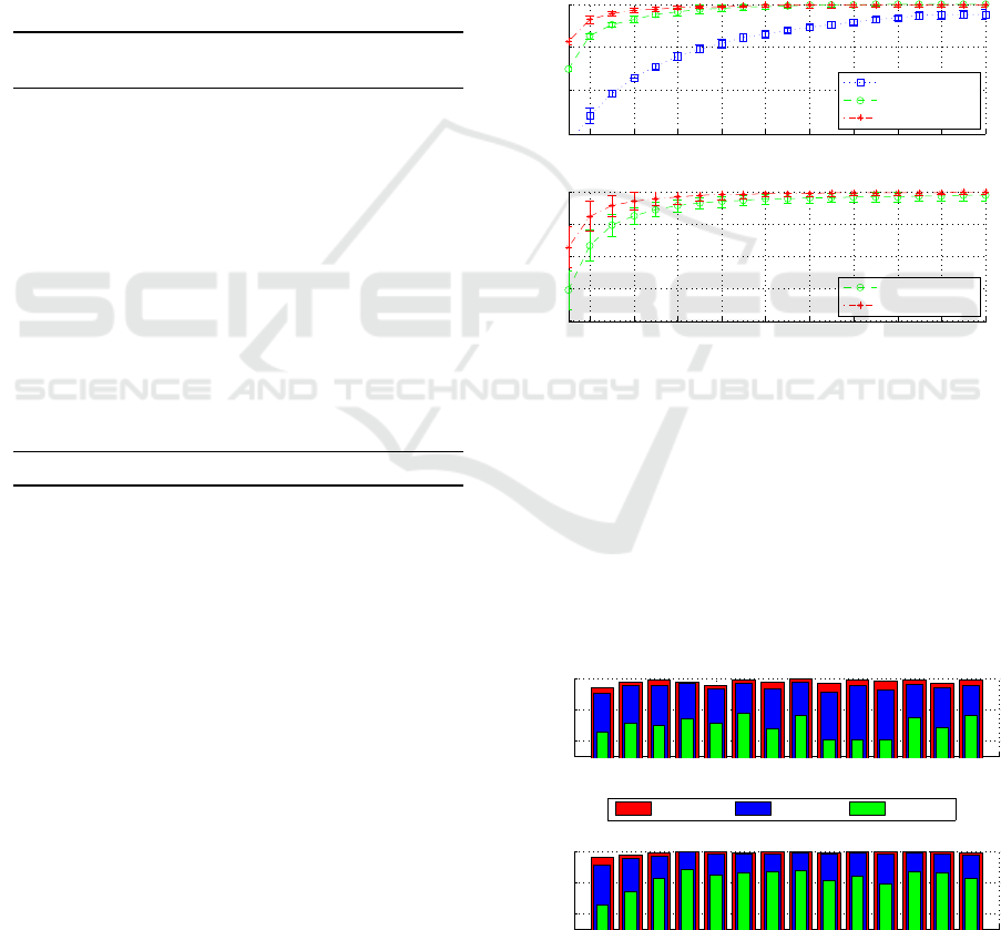
test set. Figure 3(a) shows graphically the accuracy
vs. number of sentences for a particular course with
ID 3. The accuracies are obtained from 3 different
methods, SRI uniqram, 4-gram and NNLM 4-gram.
The number of randomly selected sentences is in the
range of 1 to 20, and for each particular number of
sentences, 100 trials were performed and the mean ac-
curacies with standard deviations are shown in the fig-
ure. As mentioned earlier in Sec. 2, courses with ID
7 and 16 were taught by the same instructor, so these
two courses are excluded and 14 courses/instructors
are used to compute their 16-way classification ac-
curacies. Figure 3(b) demonstrates the mean accu-
racy over these 14 courses. SRI 4-gram and NNLM
4-gram achieve similar accuracy and variation. How-
ever, the NNLM 4-gram is slightly more accurate than
the SRI 4-gram.
2 4 6 8 10 12 14 16 18 20
0.4
0.6
0.8
1
No. of sentences
Avgerage Accuracy
1−of−16 Classfication Accuracy vs. Text Length, Course ID: 3
unigram (SRI)
4gram (SRI)
4gram (NNLM)
2 4 6 8 10 12 14 16 18 20
0.6
0.7
0.8
0.9
1
No. of sentences
Course Avgerage Accuracy
1−of−16 Course Average Classfication Accuracy vs. Text Length
4gram (SRI)
4gram (NNLM)
Figure 3: Individual (a) and mean (b) accuracies vs. text
length in terms of the number of sentences.
Figure 4 again compares the accuracies from these
two models. It provides the accuracies of 3 difficulty
stages, given 1, 5, or 10 test sentences. Both LMs per-
form differently along all course/instructor datasets.
However, NNLM 4-gram is on average slightly bet-
ter than SRI 4-gram, especially when the number of
sentences is less.
0 5 10 15
0.6
0.8
1
Dataset index (C)
Accuracy
SRI 4−gram
10 sentences 5 sentences 1 sentence
0 5 10 15
0.6
0.8
1
Dataset index (C)
Accuracy
NNLM 4−gram
Figure 4: Accuracies at 3 stages differed by text length for
each of the 14 courses. The 2 courses taught by the same
instructor are excluded.
ICPRAM 2016 - International Conference on Pattern Recognition Applications and Methods
602

Besides classification accuracy, the confusion be-
tween different course/instructors is also investigated.
Figure 5 shows the confusion matrices for all 16
courses/instructors, computed with only one ran-
domly picked test sentence for both methods. The
probabilities are all in log scale for better visualiza-
tion. The confusion value for the ith row and jth
column is the log probability of assigning the ith
course/instructor as the jth one. Since course 7 and
16 were taught by the same instructor, it is not sur-
prising that the values for (7,16) and (16,7) are larger
than the others in the same row. In addition, instruc-
tors who taught the courses in the same field, such as
courses 1,2 (Algorithm) and courses 11,12,13 (NLP)
are more likely to be confused with each other. So
the topic of the text does play a big role in authorship
attribution. Since the NNLM 4-gram assigns higher
values than the SRI the 4-gram for (7,16) and (16,7),
it is more biased towards the author rather than the
content in that sense.
12345678910111213141516
1 ‐0.4 ‐2.6 ‐3.5 ‐4.7 ‐4.2 ‐4.5 ‐3.6 ‐3.9 ‐4.2 ‐3.6 ‐3.8 ‐3.7 ‐3.9 ‐4.3 ‐4.9 ‐3.6
2 ‐3.2 ‐0.3 ‐4.3 ‐4.8 ‐4.6 ‐4.9 ‐3.9 ‐4.1 ‐3.9 ‐3.9 ‐4.5 ‐4.3 ‐4.2 ‐4.5 ‐3.8 ‐3.7
3 ‐4.3 ‐4.5 ‐0.2 ‐5.6 ‐4.4 ‐3.8 ‐4.7 ‐5.1 ‐3.7 ‐4.5 ‐5.2 ‐5.0 ‐4.4 ‐5.3 ‐4.5 ‐3.8
4
‐4.9 ‐5.5 ‐4.7 ‐0.1 ‐4.4 ‐5.4 ‐6.1 ‐5.5 ‐4.8 ‐4.4 ‐4.7 ‐5.8 ‐4.6 ‐5.6 ‐5.9 ‐3.9
5 ‐4.5 ‐4.8 ‐4.2 ‐4.5 ‐0.2 ‐5.0 ‐5.5 ‐5.1 ‐5.1 ‐4.3 ‐4.5 ‐4.7 ‐4.5 ‐5.0 ‐5.0 ‐3.8
6 ‐5.1 ‐5.1 ‐4.0 ‐5.5 ‐4.9 ‐0.1 ‐5.7 ‐4.4 ‐4.7 ‐4.2 ‐4.7 ‐5.2 ‐4.2 ‐5.3 ‐5.1 ‐4.3
7 ‐3.3
‐3.0 ‐3.8 ‐4.5 ‐4.5 ‐4.3 ‐0.6 ‐4.4 ‐3.8 ‐3.4 ‐3.8 ‐4.1 ‐4.7 ‐4.3 ‐3.4 ‐2.1
8 ‐5.1 ‐4.7 ‐4.7 ‐5.5 ‐4.8 ‐4.7 ‐5.1 ‐0.1 ‐4.4 ‐4.2 ‐5.1 ‐4.8 ‐4.7 ‐4.9 ‐5.3 ‐4.2
9 ‐5.4 ‐5.3 ‐4.6 ‐5.5 ‐5.4 ‐5.7 ‐5.7 ‐4.5 ‐0.1 ‐4.4 ‐4.8 ‐5.2 ‐4.3 ‐5.4 ‐5.1 ‐3.6
10 ‐4.1 ‐4.7
‐4.0 ‐4.5 ‐5.4 ‐5.4 ‐4.4 ‐4.2 ‐4.3 ‐0.2 ‐4.9 ‐5.2 ‐4.6 ‐4.8 ‐4.3 ‐3.3
11 ‐4.4 ‐5.0 ‐4.5 ‐4.3 ‐4.0 ‐5.8 ‐4.9 ‐5.8 ‐4.2 ‐4.5 ‐0.2 ‐4.7 ‐4.2 ‐4.5 ‐5.8 ‐4.0
12 ‐4.0 ‐5.0 ‐3.9 ‐5.1 ‐4.0 ‐4.7 ‐5.4 ‐4.4 ‐4.1 ‐4.0 ‐4.0 ‐0.2 ‐4.0 ‐4.7 ‐4.5 ‐3.7
13 ‐5.4 ‐4.7 ‐4.4
‐4.2 ‐4.8 ‐4.9 ‐5.5 ‐4.7 ‐4.8 ‐4.8 ‐4.7 ‐5.5 ‐0.1 ‐5.3 ‐5.1 ‐3.9
14 ‐4.5 ‐5.0 ‐4.7 ‐6.2 ‐4.7 ‐5.5 ‐5.6 ‐4.9 ‐4.6 ‐4.0 ‐4.2 ‐4.7 ‐4.7 ‐0.1 ‐5.6 ‐4.1
15 ‐4.5 ‐4.6 ‐3.9 ‐4.8 ‐4.8 ‐5.1 ‐4.7 ‐4.3 ‐4.7 ‐4.1 ‐4.7 ‐4.7 ‐4.5 ‐5.1 ‐0.2 ‐3.9
16 ‐3.4 ‐3.3 ‐3.4 ‐5.0
‐4.6 ‐5.6 ‐2.5 ‐4.9 ‐3.6 ‐2.7 ‐3.8 ‐4.2 ‐3.8 ‐4.6 ‐3.9 ‐0.5
12345678910111213141516
1 ‐0.4 ‐2.3 ‐4.3 ‐5.2 ‐3.7 ‐4.5 ‐3.8 ‐4.2 ‐4.0 ‐3.7 ‐4.5 ‐4.1 ‐4.0 ‐4.2 ‐4.4 ‐3.3
2 ‐3.1 ‐0.3 ‐3.8 ‐4.9 ‐4.3 ‐4.5 ‐4.0 ‐4.0 ‐4.0 ‐3.7 ‐4.0 ‐4.5 ‐4.0 ‐4.4 ‐3.7 ‐3.5
3 ‐4.2 ‐4.1 ‐0.4 ‐3.5 ‐
3.9 ‐4.1 ‐4.1 ‐4.2 ‐4.1 ‐3.4 ‐4.3 ‐4.4 ‐4.0 ‐4.1 ‐4.8 ‐2.9
4 ‐4.0 ‐3.9 ‐3.9 ‐0.3 ‐3.5 ‐4.3 ‐4.4 ‐4.7 ‐3.8 ‐4.2 ‐4.5 ‐4.6 ‐3.9 ‐4.1 ‐4.2 ‐3.8
5 ‐3.9 ‐3.9 ‐4.0 ‐3.8 ‐0.3 ‐4.0 ‐3.8 ‐4.7 ‐4.0 ‐4.5 ‐3.4 ‐3.9 ‐3.6 ‐4.2 ‐4.0 ‐4.3
6 ‐4.4 ‐4.0 ‐3.8 ‐4.2 ‐4.2 ‐
0.3 ‐4.5 ‐3.9 ‐3.8 ‐4.7 ‐4.4 ‐4.9 ‐4.1 ‐4.3 ‐3.9 ‐4.9
7 ‐4.2 ‐3.9 ‐3.5 ‐4.2 ‐4.6 ‐4.9 ‐0.3 ‐4.7 ‐4.4 ‐3.6 ‐3.9 ‐5.0 ‐4.3 ‐4.3 ‐4.8 ‐2.
8
8 ‐3.7 ‐3.0 ‐4.4 ‐5.1 ‐4.6 ‐3.7 ‐3.9 ‐0.4 ‐3.3 ‐3.6 ‐3.9 ‐4.6 ‐4.1 ‐3.8 ‐3.7 ‐4.0
9 ‐4.5 ‐3.4 ‐4.4 ‐5.5 ‐4.8 ‐4.4 ‐4.1 ‐4.3 ‐0.3 ‐3.5 ‐4.4 ‐4.7 ‐3.9 ‐4.1 ‐4.5 ‐3.8
10 ‐3.3 ‐3.1 ‐3.7 ‐4.7 ‐4.3 ‐4.7 ‐3.5 ‐3.8 ‐3.4 ‐0.5 ‐4.2 ‐4.1 ‐4.5 ‐4.0 ‐3.5 ‐2.6
11 ‐
3.9 ‐3.2 ‐4.1 ‐4.8 ‐3.0 ‐4.7 ‐3.8 ‐4.9 ‐3.4 ‐4.5 ‐0.5 ‐3.0 ‐3.0 ‐3.4 ‐4.3 ‐3.8
12 ‐3.5 ‐3.2 ‐4.2 ‐4.4 ‐3.3 ‐4.3 ‐4.0 ‐4.5 ‐3.5 ‐4.1 ‐2.8 ‐0.5 ‐3.4 ‐3.6 ‐3.7 ‐3.7
13 ‐4.3 ‐3.5 ‐4.4 ‐5.0 ‐3.8 ‐4.2 ‐4.7 ‐5.0 ‐3.6 ‐4.9 ‐3.4 ‐4.1 ‐0.3 ‐4.3 ‐3.8 ‐4.2
14 ‐3.9 ‐
3.0 ‐4.8 ‐4.7 ‐4.0 ‐4.0 ‐3.8 ‐4.6 ‐3.3 ‐4.0 ‐3.7 ‐3.8 ‐3.8 ‐0.4 ‐4.0 ‐4.4
15 ‐4.2 ‐3.4 ‐4.5 ‐4.6 ‐4.3 ‐4.4 ‐3.7 ‐4.5 ‐4.1 ‐4.1 ‐4.2 ‐4.2 ‐4.2 ‐4.5 ‐0.3 ‐4.2
16 ‐4.4 ‐4.5 ‐4.1 ‐4.2 ‐4.5 ‐6.0 ‐3.7 ‐4.9 ‐4.7 ‐3.7 ‐4.4 ‐5.2 ‐4.8 ‐5.2 ‐5.2 ‐0.2
(a)
12345678910111213141516
1 ‐0.4 ‐2.6 ‐3.5 ‐4.7 ‐4.2 ‐4.5 ‐3.6 ‐3.9 ‐4.2 ‐3.6 ‐3.8 ‐3.7 ‐3.9 ‐4.3 ‐4.9 ‐3.6
2 ‐3.2 ‐0.3 ‐4.3 ‐4.8 ‐4.6 ‐4.9 ‐3.9 ‐4.1 ‐3.9 ‐3.9 ‐4.5 ‐4.3 ‐4.2 ‐4.5 ‐3.8 ‐3.7
3 ‐4.3 ‐4.5 ‐0.2 ‐5.6 ‐4.4 ‐3.8 ‐4.7 ‐5.1 ‐3.7 ‐4.5 ‐5.2 ‐5.0 ‐4.4 ‐5.3 ‐4.5 ‐3.8
4
‐4.9 ‐5.5 ‐4.7 ‐0.1 ‐4.4 ‐5.4 ‐6.1 ‐5.5 ‐4.8 ‐4.4 ‐4.7 ‐5.8 ‐4.6 ‐5.6 ‐5.9 ‐3.9
5 ‐4.5 ‐4.8 ‐4.2 ‐4.5 ‐0.2 ‐5.0 ‐5.5 ‐5.1 ‐5.1 ‐4.3 ‐4.5 ‐4.7 ‐4.5 ‐5.0 ‐5.0 ‐3.8
6 ‐5.1 ‐5.1 ‐4.0 ‐5.5 ‐4.9 ‐0.1 ‐5.7 ‐4.4 ‐4.7 ‐4.2 ‐4.7 ‐5.2 ‐4.2 ‐5.3 ‐5.1 ‐4.3
7 ‐3.3
‐3.0 ‐3.8 ‐4.5 ‐4.5 ‐4.3 ‐0.6 ‐4.4 ‐3.8 ‐3.4 ‐3.8 ‐4.1 ‐4.7 ‐4.3 ‐3.4 ‐2.1
8 ‐5.1 ‐4.7 ‐4.7 ‐5.5 ‐4.8 ‐4.7 ‐5.1 ‐0.1 ‐4.4 ‐4.2 ‐5.1 ‐4.8 ‐4.7 ‐4.9 ‐5.3 ‐4.2
9 ‐5.4 ‐5.3 ‐4.6 ‐5.5 ‐5.4 ‐5.7 ‐5.7 ‐4.5 ‐0.1 ‐4.4 ‐4.8 ‐5.2 ‐4.3 ‐5.4 ‐5.1 ‐3.6
10 ‐4.1 ‐4.7
‐4.0 ‐4.5 ‐5.4 ‐5.4 ‐4.4 ‐4.2 ‐4.3 ‐0.2 ‐4.9 ‐5.2 ‐4.6 ‐4.8 ‐4.3 ‐3.3
11 ‐4.4 ‐5.0 ‐4.5 ‐4.3 ‐4.0 ‐5.8 ‐4.9 ‐5.8 ‐4.2 ‐4.5 ‐0.2 ‐4.7 ‐4.2 ‐4.5 ‐5.8 ‐4.0
12 ‐4.0 ‐5.0 ‐3.9 ‐5.1 ‐4.0 ‐4.7 ‐5.4 ‐4.4 ‐4.1 ‐4.0 ‐4.0 ‐0.2 ‐4.0 ‐4.7 ‐4.5 ‐3.7
13 ‐5.4 ‐4.7 ‐4.4
‐4.2 ‐4.8 ‐4.9 ‐5.5 ‐4.7 ‐4.8 ‐4.8 ‐4.7 ‐5.5 ‐0.1 ‐5.3 ‐5.1 ‐3.9
14 ‐4.5 ‐5.0 ‐4.7 ‐6.2 ‐4.7 ‐5.5 ‐5.6 ‐4.9 ‐4.6 ‐4.0 ‐4.2 ‐4.7 ‐4.7 ‐0.1 ‐5.6 ‐4.1
15 ‐4.5 ‐4.6 ‐3.9 ‐4.8 ‐4.8 ‐5.1 ‐4.7 ‐4.3 ‐4.7 ‐4.1 ‐4.7 ‐4.7 ‐4.5 ‐5.1 ‐0.2 ‐3.9
16 ‐3.4 ‐3.3 ‐3.4 ‐5.0
‐4.6 ‐5.6 ‐2.5 ‐4.9 ‐3.6 ‐2.7 ‐3.8 ‐4.2 ‐3.8 ‐4.6 ‐3.9 ‐0.5
12345678910111213141516
1 ‐0.4 ‐2.3 ‐4.3 ‐5.2 ‐3.7 ‐4.5 ‐3.8 ‐4.2 ‐4.0 ‐3.7 ‐4.5 ‐4.1 ‐4.0 ‐4.2 ‐4.4 ‐3.3
2 ‐3.1 ‐0.3 ‐3.8 ‐4.9 ‐4.3 ‐4.5 ‐4.0 ‐4.0 ‐4.0 ‐3.7 ‐4.0 ‐4.5 ‐4.0 ‐4.4 ‐3.7 ‐3.5
3 ‐4.2 ‐4.1 ‐0.4 ‐3.5 ‐
3.9 ‐4.1 ‐4.1 ‐4.2 ‐4.1 ‐3.4 ‐4.3 ‐4.4 ‐4.0 ‐4.1 ‐4.8 ‐2.9
4 ‐4.0 ‐3.9 ‐3.9 ‐0.3 ‐3.5 ‐4.3 ‐4.4 ‐4.7 ‐3.8 ‐4.2 ‐4.5 ‐4.6 ‐3.9 ‐4.1 ‐4.2 ‐3.8
5 ‐3.9 ‐3.9 ‐4.0 ‐3.8 ‐0.3 ‐4.0 ‐3.8 ‐4.7 ‐4.0 ‐4.5 ‐3.4 ‐3.9 ‐3.6 ‐4.2 ‐4.0 ‐4.3
6 ‐4.4 ‐4.0 ‐3.8 ‐4.2 ‐4.2 ‐
0.3 ‐4.5 ‐3.9 ‐3.8 ‐4.7 ‐4.4 ‐4.9 ‐4.1 ‐4.3 ‐3.9 ‐4.9
7 ‐4.2 ‐3.9 ‐3.5 ‐4.2 ‐4.6 ‐4.9 ‐0.3 ‐4.7 ‐4.4 ‐3.6 ‐3.9 ‐5.0 ‐4.3 ‐4.3 ‐4.8 ‐2.
8
8 ‐3.7 ‐3.0 ‐4.4 ‐5.1 ‐4.6 ‐3.7 ‐3.9 ‐0.4 ‐3.3 ‐3.6 ‐3.9 ‐4.6 ‐4.1 ‐3.8 ‐3.7 ‐4.0
9 ‐4.5 ‐3.4 ‐4.4 ‐5.5 ‐4.8 ‐4.4 ‐4.1 ‐4.3 ‐0.3 ‐3.5 ‐4.4 ‐4.7 ‐3.9 ‐4.1 ‐4.5 ‐3.8
10 ‐3.3 ‐3.1 ‐3.7 ‐4.7 ‐4.3 ‐4.7 ‐3.5 ‐3.8 ‐3.4 ‐0.5 ‐4.2 ‐4.1 ‐4.5 ‐4.0 ‐3.5 ‐2.6
11 ‐
3.9 ‐3.2 ‐4.1 ‐4.8 ‐3.0 ‐4.7 ‐3.8 ‐4.9 ‐3.4 ‐4.5 ‐0.5 ‐3.0 ‐3.0 ‐3.4 ‐4.3 ‐3.8
12 ‐3.5 ‐3.2 ‐4.2 ‐4.4 ‐3.3 ‐4.3 ‐4.0 ‐4.5 ‐3.5 ‐4.1 ‐2.8 ‐0.5 ‐3.4 ‐3.6 ‐3.7 ‐3.7
13 ‐4.3 ‐3.5 ‐4.4 ‐5.0 ‐3.8 ‐4.2 ‐4.7 ‐5.0 ‐3.6 ‐4.9 ‐3.4 ‐4.1 ‐0.3 ‐4.3 ‐3.8 ‐4.2
14 ‐3.9 ‐
3.0 ‐4.8 ‐4.7 ‐4.0 ‐4.0 ‐3.8 ‐4.6 ‐3.3 ‐4.0 ‐3.7 ‐3.8 ‐3.8 ‐0.4 ‐4.0 ‐4.4
15 ‐4.2 ‐3.4 ‐4.5 ‐4.6 ‐4.3 ‐4.4 ‐3.7 ‐4.5 ‐4.1 ‐4.1 ‐4.2 ‐4.2 ‐4.2 ‐4.5 ‐0.3 ‐4.2
16 ‐4.4 ‐4.5 ‐4.1 ‐4.2 ‐4.5 ‐6.0 ‐3.7 ‐4.9 ‐4.7 ‐3.7 ‐4.4 ‐5.2 ‐4.8 ‐5.2 ‐5.2 ‐0.2
(b)
Figure 5: Course/instructor confusion matrices (16×16) for
SRI 4-gram (a) and NNLM 4-gram (b).
5 CONCLUSION AND FUTURE
WORK
This paper investigates authorship attribution using
NNLM. The experimental setup for NNLM is detailed
with mathematical elaboration. The results in terms
of LM fitness in perplexity, classification accuracies,
and confusion scores are promising, compared with
the baseline N-gram methods. The performance is
very competitive to the state-of-the-art, in terms of
classification accuracy and testing sensitivity, i.e. the
length of test text used in order to achieve confident
results. From the previous work listed in Sec. 1, the
best reported results to date achieved either 95% ac-
curacy on a similar author pool size, or 50% ∼ 60%
with 100+ authors and limited training date per au-
thor. As it is shown in Figure 4, our work achieves
nearly perfect accuracies if more than 10 test sen-
tences are given.
However, since both the SRI baseline and NNLM
methods achieves nearly perfect accuracies with only
limited test data, the current database may not be suf-
ficiently large and challenging, probably due to the
consistency between the training and the test sets and
the contribution from the topic distinction. In the fu-
ture, the algorithm should be tested using datasets
with larger author set sizes and greater styling simi-
larities.
Since purely topic-neutral text data may not even
exist (Luyckx, 2011), developing general author LMs
with mixed-topic data, and then adapting them to par-
ticular topics may also be desirable. It could be partic-
ularly helpful when the topics of text data is available.
To compensate the relatively small size of the training
set, LMs may also be trained with a group of authors
and then adapt to the individuals.
Because the NNLM assigns a unique representa-
tion for a single word, it is difficult to model words
with multiple meanings (Mnih, 2010). Thus, com-
bining the NNLM and N-gram models might be ben-
eficial. The recurrent NNLM, which captures more
context size than the current feed-forward model
(Mikolov et al., 2010), may also be worth exploring.
ACKNOWLEDGEMENTS
The authors would like to thank Coursera Incorpora-
tion for providing the course transcript datasets for the
research in this paper.
Domain Specific Author Attribution based on Feedforward Neural Network Language Models
603

REFERENCES
Bengio, Y., Ducharme, R., Vincent, P., and Janvin, C.
(2003). A neural probabilistic language model. The
Journal of Machine Learning Research, 3:1137–1155.
Bishop, C. M. (1995). Neural networks for pattern recog-
nition. Oxford university press.
Coyotl-Morales, R. M., Villase
˜
nor-Pineda, L., Montes-y
G
´
omez, M., and Rosso, P. (2006). Authorship attri-
bution using word sequences. In Progress in Pattern
Recognition, Image Analysis and Applications, pages
844–853. Springer.
Ebrahimpour, M., Putnin¸
ˇ
s, T. J., Berryman, M. J., Allison,
A., Ng, B. W.-H., and Abbott, D. (2013). Automated
authorship attribution using advanced signal classifi-
cation techniques. PloS one, 8(2):e54998.
Ge, Z. and Sun, Y. (2015). Sleep stages classification us-
ing neural networks with multi-channel neural data.
In Brain Informatics and Health, pages 306–316.
Springer.
Hinton, G., Deng, L., Yu, D., Dahl, G. E., Mohamed, A.-
r., Jaitly, N., Senior, A., Vanhoucke, V., Nguyen, P.,
Sainath, T. N., et al. (2012). Deep neural networks for
acoustic modeling in speech recognition: The shared
views of four research groups. Signal Processing
Magazine, IEEE, 29(6):82–97.
Juola, P. (2006). Authorship attribution. Foundations and
Trends in information Retrieval, 1(3):233–334.
Ke
ˇ
selj, V., Peng, F., Cercone, N., and Thomas, C. (2003).
N-gram-based author profiles for authorship attribu-
tion. In Proceedings of the conference pacific asso-
ciation for computational linguistics, PACLING, vol-
ume 3, pages 255–264.
Koppel, M., Schler, J., and Argamon, S. (2009). Compu-
tational methods in authorship attribution. Journal
of the American Society for information Science and
Technology, 60(1):9–26.
Krizhevsky, A., Sutskever, I., and Hinton, G. E. (2012). Im-
agenet classification with deep convolutional neural
networks. In Advances in neural information process-
ing systems, pages 1097–1105.
Luyckx, K. (2011). Scalability issues in authorship attribu-
tion. ASP/VUBPRESS/UPA.
Luyckx, K. and Daelemans, W. (2008). Authorship attri-
bution and verification with many authors and limited
data. In Proceedings of the 22nd International Confer-
ence on Computational Linguistics-Volume 1, pages
513–520. Association for Computational Linguistics.
Mikolov, T., Karafi
´
at, M., Burget, L., Cernock
`
y, J., and
Khudanpur, S. (2010). Recurrent neural network
based language model. In INTERSPEECH 2010,
Makuhari, Chiba, Japan, September 26-30, 2010,
pages 1045–1048.
Mnih, A. (2010). Learning Distributed Representations
for Statistical Language Modelling and Collaborative
Filtering. PhD thesis, University of Toronto.
Mnih, A. and Hinton, G. (2007). Three new graphical mod-
els for statistical language modelling. In Proceed-
ings of the 24th international conference on Machine
learning, pages 641–648. ACM.
Porter, M. F. (1980). An algorithm for suffix stripping. Pro-
gram, 14(3):130–137.
Seroussi, Y., Zukerman, I., and Bohnert, F. (2011). Author-
ship attribution with latent dirichlet allocation. In Pro-
ceedings of the fifteenth conference on computational
natural language learning, pages 181–189. Associa-
tion for Computational Linguistics.
Socher, R., Lin, C. C., Manning, C., and Ng, A. Y. (2011).
Parsing natural scenes and natural language with re-
cursive neural networks. In Proceedings of the 28th
international conference on machine learning (ICML-
11), pages 129–136.
Stamatatos, E. (2009). A survey of modern authorship attri-
bution methods. Journal of the American Society for
information Science and Technology, 60(3):538–556.
Stolcke, A. et al. (2002). Srilm-an extensible language mod-
eling toolkit. In INTERSPEECH.
ICPRAM 2016 - International Conference on Pattern Recognition Applications and Methods
604
