
A Formal Approach to Anomaly Detection
Andr´e Eriksson and Hedvig Kjellstr¨om
Computer Vision and Active Perception Lab, KTH Royal Institute of Technology, Stockholm, Sweden
Keywords:
Anomaly Detection, Formal Methods, Model Selection.
Abstract:
While many advances towards effective anomaly detection techniques targeting specific applications have been
made in recent years, little work has been done to develop application-agnostic approaches to the subject. In
this article, we present such an approach, in which anomaly detection methods are treated as formal, structured
objects. We consider a general class of methods, with an emphasis on methods that utilize structural properties
of the data they operate on. For this class of methods, we develop a decomposition into sub-methods—simple,
restricted objects, which may be reasoned about independently and combined to form methods. As we show,
this formalism enables the construction of software that facilitates formulating, implementing, evaluating, as
well as algorithmically finding and calibrating anomaly detection methods.
1 INTRODUCTION
Anomaly detection tasks are encountered in many
areas of science, technology, and business, and au-
tomated anomaly detection methods are indispens-
able in many applications, such as intrusion detec-
tion and fraud detection (Lazarevic et al., 2003; Phua
et al., 2010). As manual analysis of the ever growing
datasets encounteredin many application domains be-
comes increasingly difficult, the need for such meth-
ods can be expected to grow.
For this need to be effectively met, approaches
that enable researchers and organizations to effec-
tively develop and implement appropriate methods
are required.
While there are excellent tools available for cer-
tain applications (Twitter, 2015; Etsy, 2015), there is
a notable lack of application-agnostic tools and ap-
proaches.
Considering the disparate nature of data encoun-
tered in applications, and the often subjective notion
of what constitutes an anomaly, it seems unlikely that
specific methods that work well across a majority of
applications can be found. A more viable approach
might be to instead focus on developing application-
agnostic tools that facilitate formulating, implement-
ing, evaluating, or calibrating methods.
We believe that taking a formal, high-level ap-
proach to the subject—where the focus is on what can
be said about anomaly detection methods in general,
rather than in the context of any specific application
or task—is a vital step towards this goal.
The aim of this article is to present a particular
such approach—where methods are treated as formal
objects, which map datasets to solutions (i.e. a col-
lection of anomaly scores, or a set of ‘most anoma-
lous’ items), and which may be decomposed into
sub-methods that may in turn be recombined into
methods—and to demonstrate the utility of this ap-
proach in reaching the goals outlined above.
We target a general class of methods—with a fo-
cus on methods that utilize the structure of the dataset
to find contextual or collective anomalies—for which
we develop a formalism for decomposing methods
into a collection of such sub-methods, amenable to
being shared between applications involving similar
types of data.
This enables an approach to developing methods
where the principal consideration is the collection of
applicable sub-methods (as constrained by the tar-
geted task). These sub-methods may then be com-
bined to form methods (either manually or algorith-
mically) until one that accurately solves the task at
hand is found.
To demonstrate the utility of this approach, we ap-
ply it to a number of tasks involving sequences, as
well as to finding and calibrating methods for such
tasks (given a collection of sub-methods and labeled
testing data).
2 RELATED WORK
Throughout the years, many anomaly detection
Eriksson, A. and Kjellström, H.
A Formal Approach to Anomaly Detection.
DOI: 10.5220/0005710803170326
In Proceedings of the 5th International Conference on Pattern Recognition Applications and Methods (ICPRAM 2016), pages 317-326
ISBN: 978-989-758-173-1
Copyright
c
2016 by SCITEPRESS – Science and Technology Publications, Lda. All rights reserved
317

methods and applications has been studied. Plenty of
surveys and books which discuss these in detail have
been published (Hodge and Austin, 2004; Agyemang
et al., 2006; Chandola et al., 2009; Fu, 2011).
To our knowledge, the formal, method-centric ap-
proach we take to anomaly detection is unique. How-
ever, there have been a few attempts to provide a gen-
eral treatment of anomaly detection in relation to spe-
cific applications. For instance, in (Chandola, 2009),
a high-level, formal discussion of common anomaly
detection problems for sequences is presented. We
build on this approach, taking it further and general-
izing it to other types of tasks and data.
Our discussion of anomaly detection in sequences
shows how diverse applications and methods related
to sequences can be reconciled (Chandola et al., 2012;
Chandola, 2009; Fu, 2011) and treated coherently.
We discuss a few specific tasks, including the de-
tection of point anomalies (individual anomalous ele-
ments, also referred to as outliers) (Fox, 1972; Abra-
ham and Chuang, 1989; Abraham and Box, 1979;
Galeano et al., 2006; Tsay et al., 2000), novelties
(previously unseen elements) (Markou and Singh,
2003a; Markou and Singh, 2003b; Ma and Perkins,
2003), elements anomalous with regard to nearby el-
ements (Basu and Meckesheimer, 2007) and anoma-
lous subsequences (Keogh et al., 2005; Keogh et al.,
2007; Fu et al., 2006).
3 GENERALITY
When attempting to provide a formal basis for a con-
cept as broad as anomaly detection methods, it is vital
that care is taken to ensure that the breadth of the con-
cept is captured by the resulting formalism.
In a widely cited survey of the subject, Chandola
et al. (Chandola et al., 2009) discuss a few key aspects
of anomaly detection tasks: the nature of the data and
the types of anomalies involved, the expected solution
format, and the type of supervision employed. Our
aim is to provide a formalism which captures or gen-
eralizes these three aspects.
First, we formulate our formalism in a data- and
solution-agnostic manner, so its applicability is inde-
pendent of the nature of data and solutions.
Second, we target a general type of anomalies.
Most methods are focused on detecting point anoma-
lies—individual elements anomalous compared to the
rest of the rest of the data. Such methods are appropri-
ate for unstructured data (i.e. data in which individual
elements are not related). However, the datasets en-
countered in applications (e.g. sequences, graphs, and
spatial data) often have structure that can be exploited
to better detect anomalies.
Chandola et al. discuss two other categories of
anomalies: contextual anomalies—elements anoma-
lous compared to a context (some subset of the data;
typically ‘nearby’ elements)—and collective anoma-
lies—collections of elements anomalous compared to
the rest of the data. These can both be seen as gener-
alizations of the concept of point anomalies.
Our formalism targets a fourth such category:
collective contextual anomalies—collections of ele-
ments anomalous compared to a context—which nat-
urally generalizes the other three
1
.
An illustration of these four anomaly types is
shown in Figure 1.
Figure 1: Examples of a point anomaly (top), a contextual
anomaly (above center), a collective anomaly (below cen-
ter), and a collective contextual anomaly (bottom) in uni-
variate real-valued sequences. Anomalies are shown in light
red; appropriate contexts in black.
Third, Chandola et al. classify methods as un-
supervised, semi-supervised, or supervised based on
whether they incorporate zero, one, or two classes of
labeled training data. We formalize methods as maps
from datasets to solutions; an approach naturally
suited to expressing unsupervised methods. However,
semi-supervised and supervised methods may also be
expressed by replacing the input dataset with the dis-
joint union of the evaluation data and one or two sets
of training data.
4 SUB-METHODS
Formally, an anomaly detection method may be
treated as a mapping m : D → S, that associates with
each potential input dataset d ∈ D a solution s ∈ S,
where:
• D is an application-dependent set of well-formed
datasets (e.g. all real-valued sequences, or all po-
tential sets of users of a social network). We will
1
Contextual and point anomalies correspond to single-
element collections; for collective and point anomalies, the
context is the entire dataset.
ICPRAM 2016 - International Conference on Pattern Recognition Applications and Methods
318

Figure 2: A dataset (center right) in D = P (C × B) = P (N
2
× R), constructed by linearly combining periodic data (far left)
and data containing an anomaly (center left). We use the pattern on the far right to indicate contextual data.
assume that any dataset d is a set of items in some
application-specific set X, so
2
D ⊆ P (X).
• S is a corresponding application-dependent set
of potential solutions (e.g. all sequences of real-
valued anomaly scores, or all potential sets of
anomalous clusters of users in a social network).
For any given application, the set M = D → S cor-
responds to all potential methods.
When designing a method targeting point anoma-
lies, there are two aspects to consider: what anomaly
measure should be used to compare each item to the
rest of the data, and how the results of these compar-
isons should be aggregated to form a solution.
Targeting collective anomalies means an addi-
tional aspect must be considered: how the set of can-
didate anomalies should be selected.
When targeting contextual anomalies, one must
instead consider how a context should be associated
with each candidate anomaly.
Since our formalism targets collective contextual
anomalies, it must capture all four of these aspects.
This may be achieved by decomposing any m ∈ M
into four sub-methods, each responsible for one as-
pect. We will encode these as functions:
• The selection of candidate anomalies may be en-
coded as a function
α : D → P (D),
which maps any dataset to a set of candidate
anomalies
3
(subsets of that data; i.e. ∀x,∀y ∈
f(x) : y ⊂ x). For methods targeting point and
contextual anomalies, α produces singleton sets;
i.e. α(d) = {{x}|x ∈ d}.
• The selection of contexts may be encoded as a
function
β : D× D → D,
which maps any dataset and one of its candi-
date anomalies to the context of that candidate
2
We denote the power set of a set X by P (X).
3
Here, and in the remainder of this section, we assume
that information about the ‘original’ position of data items
in the dataset is implicitly preserved when the data is rear-
ranged or transformed. This issue is resolved in Section 5
through the requirement that the contextual data of each
item is unique.
anomaly (a subset of the dataset, disjoint with the
candidate anomaly; i.e. ∀x,∀y ⊂ x : β(x,y) ⊆ x\y).
For methods targeting point and collectiveanoma-
lies, β(x,y) = x\ y.
• The comparison of candidate anomalies and con-
texts may be encoded as a function
γ : D× D → A,
which assigns a dissimilarity score a ∈ A (where
A is some method-specific set) to any candidate
anomaly-context pair.
• The aggregation of anomaly scores may be en-
coded as a function
δ : P (D× A) → S,
which maps any collection of candidate anomaly-
dissimilarity score pairs to a solution.
Any tuple (α,β,γ, δ) (for given S, D, and A) may
be combined
4
to form an m ∈ M. Conversely, any m ∈
M may be defined
5
as a tuple m = (D,S,A,α, β,γ,δ).
For any given application, appropriate methods
may be designed by reasoning about which choices
of these sub-methods are applicable.
As an illustration of this approach, consider an
application involving grids of real-valued data con-
taining collective contextual anomalies (regions of the
grid, anomalous with regard to their surroundings), as
illustrated in Figure 2. Assume that the desired so-
lution format is a grid of real-valued anomaly scores;
i.e. S = D. What choices of sub-methods might be
suitable?
First, α should produce candidate anomalies
roughly on the scale of the anomalies we wish to
capture. For instance, an α that produces non-
overlapping square regions of size 6-by-6 may be em-
ployed:
D ∋
α
7−→ {
, ,... } ∈ P (D)
4
Specifically by—for d ∈ D—letting X = α(d),
Y = {(x, β(x, d)) | x ∈ X}, Z = {(x,γ(x,y)) | (x,y) ∈ Y}, and
m(d) = δ(Z).
5
Note that this implies no loss of generality; any
m : D → S may be encoded by e.g. letting A = S, α(d) =
{d}, γ(d,y) = m(d), and δ({s}) = s.
A Formal Approach to Anomaly Detection
319

Second, β should produce as context some appro-
priately sized neighborhoodof the candidate anomaly,
such as the union of all adjacent such square regions:
D× D ∋
,
!
β
7−→
∈ D,
,
!
β
7−→
,.. .
Third, γ may be selected to compute the mean
value of the items in the candidate anomaly, and the
mean values in each 6-by-6 region of the context, and
produce as anomaly score the mean absolute differ-
ence between the former and the latter (this means
that A = R)
6
:
D× D ∋
,
γ
7−→
∈ A,
,
!
γ
7−→
,.. .
Finally, δ should be selected to associate with each
element the anomaly score of the candidate anomaly
to which it belongs:
P (D× A) ∋ {(
, ),... }
δ
7−→ ∈ S
It would be an easy task to construct software that
takes implementations of α, β, γ, and δ and combines
them into a corresponding method implementation.
Such software might be useful in constructing, cali-
brating, or evaluating methods.
However, its utility would be limited by the fact
that α, β, γ, and δ are all formulated in terms of D,
and would thus have to be implemented anew for each
new application.
If the sub-methods could be defined such that
implementations could be shared between applica-
tions with similar (rather than identical) data, soft-
ware could then be coupled with a library of imple-
mented sub-methods, drastically increasing its utility.
5 CONTEXTUAL AND
BEHAVIORAL ATTRIBUTES
To accomplish this, we may instead define our sub-
methods to operate on either behavioral or contextual
attributes of the data.
6
We illustrate values in R as colored squares. To im-
prove the clarity of the presentation, we normalize anomaly
scores so that the most and least anomalous values of our
example are colored red and green, respectively.
By contextual attributes, we mean attributes
which identify and relate individualitems of a dataset,
such as the position in spatial data, the index in se-
quential data, or the vertex in graph data. These may
be thought of as ‘tags’ for each item in a dataset,
and must be unique. Behavioral attributes, are any
other attributes. These are ideally relevant only to the
anomaly measure.
Accordingly, we will henceforth assume that D
may be decomposed as D = P (C × B), where C and
B are (application-specific) sets of contextual and be-
havioral data, respectively. In our example applica-
tion, these may be represented as C = N
2
(capturing
the two-dimensional nature of the data) and B = R.
The sub-methodsmay then be replaced as follows:
• Behavioral data should be irrelevant when select-
ing candidate anomalies, so α may be replaced by
α
′
: P (C) → P (P (C)),
which operates on contextual data rather than on
the full dataset.
• Similarly, β may be replaced by
β
′
: P (C) × P (C) → P (C).
• When targeting point or contextual anomalies, γ
may be replaced with a function
γ
′
: B× P (B) → A,
that maps behavioral attributes of the candidate
item and the context to an anomaly score.
When targeting collective or collective contextual
anomalies, however, both contextual and behav-
ioral aspects are likely to be relevant when com-
puting the anomaly measure. Thus, replacing γ
with sub-methods operating on either C or B is
not feasible.
A better approach would be to break γ apart into
smaller sub-methods, isolating the relation of con-
textual and behavioural considerations to a single,
constrained sub-method.
Many anomaly measures compare one feature to
a set of similar features, and are not formulated to
operate on contextual data. For these, γ may be
seen as encoding two responsibilities: extracting
features from candidate anomalies and contexts,
and comparing these to form anomaly scores.
These responsibilities may be encoded as (where
F is some method-specific set of features)
ε : D× D → F × P (F), and
ζ : F × P (F) → A.
Note that the anomaly measure ζ is not coupled to
either C or B, so it is independent of D (as long as
the features it operated on can be extracted).
ICPRAM 2016 - International Conference on Pattern Recognition Applications and Methods
320

In turn, ε may be seen as encoding two respon-
sibilities: breaking the context up into a set of
items, and extracting a single feature from each
such item.
These responsibilities may be encoded separately
as
η : P (C) → P (P (C))
(note the similarity to α
′
), and
θ : D → F.
• Behavioral data should be irrelevant when aggre-
gating anomaly scores, so δ may be replaced by
δ
′
: P (P (C) × A) → S.
If S is known, δ
′
may in turn be replaced further.
Reasonably, any S should involve assigning labels
or scores either to individual items or to subsets
of the data, so we may assume that S = P (G× L),
where either G = C or G = P (C), and L is some
set of labels.
When S = P (C × L), and all candidate candidate
anomalies are singleton sets (i.e. when point or
contextual anomalies are targeted) δ
′
may be set
to
δ
′
({({c
1
},a
1
),... }) = {(c
1
,ι(a
1
)),... }
for some function ι : A → L.
Typically, either A = L = R, in which case ι may
be set as the identity function, or A = R and L =
{0,1}, in which case ι may be set as a threshold
function.
Analogously, when S = P (P (C) × L), δ
′
may be
set to
δ
′
({(C
1
,a
1
),... }) = {(C
1
,ι(a
1
)),... }.
Finally, when S = P (C × L) and there are non-
singleton candidate anomalies, δ
′
may be set to
δ
′
({(C
1
,a
1
),... }) =
n
(c
j
,κ(A
j
)) | c
j
∈
[
C
i
o
,
where A
j
= {a
k
| c
j
∈ C
k
}, i.e. for each data item,
the anomaly scores for all candidate anomalies
to which it belongs are aggregated through some
function κ : P (A) → L.
The above sub-methods allow for decompos-
ing methods to various degrees; i.e. a method
may be specified as (D,S,A,α
′
,β
′
,γ
′
,δ
′
), or
(D,S, F,A,α
′
,β
′
,η,θ,ζ, δ
′
), et cetera. Crucially,
it is an easy task to write software that constructs a
corresponding method for any such combination
7
,
7
In the interest of saving space, we elide a precise for-
mulation of how the sub-methods would be composed.
and by extension, software that can algorithmically
find appropriate methods given a set of potentially
applicable sub-methods.
For a given choice of C, the number of interest-
ing sub-methods can be rather limited (as we will see
in Section 8). Thus, implementations of a few sub-
methods may be used to handle a wide range of tasks.
As an illustration of the sub-methods proposed
above, we may consider how they may be used to re-
place the α, β, γ, and δ we applied to our example
data. To indicate contextual data, we will use the pat-
tern to the far right in Figure 2.
Our choice of α corresponds to an analogous α
′
:
P (C) ∋
α
′
7−−→ {
, ,...} ∈ P (P (C))
The same goes for our choice of β:
P (C)
2
∋
,
!
β
′
7−−→
∈ P (C)
,
!
β
′
7−−→
,.. .
Our choice of γ corresponds to an ε that produces
as features the mean value of each 6-by-6 region (so
F = R), and a ζ that computes the mean absolute dif-
ference between the feature extracted from the candi-
date anomaly and the features extracted from the con-
text:
D
2
∋
,
ε
7−→ (
,{ , , }) ∈ F ×P (F)
,
!
ε
7−→ (
,{ , ,. .. }),.. .
F × P (F) ∋ (
,{ , , })
ζ
7−→ ∈ A,
(
,{ , ,. .. })
ζ
7−→ ,.. .
In turn, this ε corresponds to an η that extracts
disjoint such square regions, and a θ that computes
the mean value of its inputs:
P (C) ∋
η
7−→ {
, , } ∈ P (P (C)),
η
7−→ {
, , ,. .. },.. .
D ∋
θ
7−→
∈ F,
θ
7−→
,.. .
Our δ may be replaced with an analogous δ
′
:
P (P (C) × A) ∋ {(
, ),...}
δ
′
7−−→
∈ S
A Formal Approach to Anomaly Detection
321

Finally, since the solution format is S = P (C× L)
for L = A = R, and we are dealing with collective con-
textual anomalies, we may utilize κ. The candidate
anomalies are disjoint, so κ should produce the single
elements of the sets it receives:
P (A) ∋ {
}
κ
7−→ ∈ L, { }
κ
7−→ ,...
6 PARAMETRIC SUB-METHODS
Assuming that D = P (C × B) and S = P (G× L), the
construction of a m ∈ M = D → S from e.g. some α
′
,
β
′
, γ
′
, and δ
′
may be seen as the application of a func-
tion
f(α
′
,β
′
,γ
′
,δ
′
) : A
′
C
× B
′
C
× Γ
′
C,B,A
× ∆
′
C,A,G,L
→ M,
where A
′
C
= P (C) → P (P (C)), et cetera.
Likewise, the construction of e.g. a γ
′
from some
ε and ζ may be seen as the application of a function
g(ε,ζ) : E
C,B,F
× Z
F,A
→ Γ
′
C,B,A
.
Taking this approach one step further, we may
consider parametric sub-methods—functions that
take some tuple of parameters and produce a sub-
method.
For instance, our choice of an α
′
that produces re-
gions of size 6-by-6 may be seen as a special case of
a parametric sub-method
α
′
rect
(w,h) : N × N → (P (N
2
) → P (P (N
2
))) = A
′
N
2
that produces regions of width w and height h.
As we will see in Sections 8 and 9, parametric sub-
methods naturally arise in applications, and are very
helpful when formulating methods as well as when
heuristically searching for appropriate methods.
7 HIGHER ORDER METHODS
Similarly, we may consider higher order methods,
which map methods to methods.
For instance, consider the function
τ : T
C
′
,B
′
,C,B
× M
C,B,G,L
× T
G,L,G
′
,L
′
→ M
C
′
,B
′
,G
′
,L
′
,
defined by
τ(t
i
,m,t
o
) = t
o
◦ m ◦ t
i
,
which takes an input transform
t
i
∈ T
C
′
,B
′
,C,B
= P (C
′
× B
′
) → P (C × B),
for some C
′
, B
′
, a method
m ∈ M
C,B,G,L
= P (C× B) → P (G× L),
and an output transform
t
o
∈ T
G,L,G
′
,L
′
= P (G× L) → P (G
′
× L
′
),
for some G
′
, L
′
, and produces a method
m
′
∈ P (C
′
× B
′
) → P (G
′
× L
′
).
Many methods found in the literature involve a
pre-analysis transformation of the data into some for-
mat more amenable to analysis, either through dimen-
sionality reduction (Ding et al., 2008) or a change of
data representation (i.e. of C or B) (Lin et al., 2007).
Such methods may be accommodated through the use
of τ together with appropriate t
i
and t
o
.
For instance, dimensionality reducing transforma-
tions may be applied to our example method to ob-
tain equivalent methods that operate on a lower di-
mensionality:
Here, t
i
,t
′
i
,t
o
,t
′
o
∈ T
Z
2
,R,Z
2
,R
and
m = τ(t
i
,m
′
,t
o
) = τ(t
i
,τ(t
′
i
,m
′′
,t
′
o
),t
o
).
Another interesting higher order method, which
may be used to combine methods into ensembles, is
µ : P (M
C,B,G,L
) ×U
G,L
→ M
C,B,G,L
, given by
µ(m,u)(d) = u({m
i
(d) | m
i
∈ m}),
where u ∈ U
G,L
= P (P (G× L)) → P (G× L) is some
function that combines solutions.
Crucially, t
i
, t
o
and u may be used analogously to
sub-methods to construct methods, either manually or
algorithmically.
8 AN APPLICATION TO
SEQUENCES
Anomaly detection tasks involving sequences
8
are
commonly encountered in applications, and have
8
We here consider only regular sequences, as opposed
to irregular time series, for whichC = R, and which may be
considered a type of one-dimensional spatial data.
ICPRAM 2016 - International Conference on Pattern Recognition Applications and Methods
322

been extensively studied. For sequences, we may let
C = N.
We will now illustrate how our approach may be
used to formulate methods through an application to
sequences. In the interest of saving space, we will
restrict our attention to S = P (G × L) = P (N × R)
(solutions which consist of real-valued per-element
anomaly scores).
First, consider the following real-valued sequence
(in D = P (N × R)):
This sequence consists of a sinusoid with added
noise, and two abnormalities: two extrema (in its lat-
ter half) and a trend of stray elements (beginning near
its middle). Either abnormality may be considered an
anomaly with regard to the (hypothetical) underlying
application, so detecting either or both might be valu-
able.
To detect the extrema, methods targeting point
anomalies may be employed. As previously dis-
cussed, when point anomalies are targeted, and G =
C, it suffices to specify γ
′
(an anomaly measure) and
ι (a method of aggregating anomaly scores). We will
restrict our consideration to A = L = R, and may thus
let ι(x) = x.
A common choice of anomaly measures are k-
nearest neighbor-basedmeasures, which for any given
candidate anomaly compute the mean distance to its k
nearest elements (for some distance measure d). We
may capture such measures through a parametric sub-
method
γ
′
kNN
(k,d) : N × (R × R → R) → (R × P (R) → R),
where γ
′
kNN
(k,d)(x,y) produces the mean of the k
smallest values in {d(x,y
i
) | y
i
∈ y}.
Applying γ
′
kNN
(3,d
E
) (for d
E
(x,y) = |x − y|) to
our sequence gives the following result (the anomaly
score is indicated through color and point size; large,
bright points indicate anomalous items):
As expected, it captures the extrema but not the
trend of stray elements. The elements of this trend
are contextual anomalies with regard to a local con-
text, which consists of all elements within some dis-
tance m of a candidate anomaly (with respect to the
sequence ordering). This may be captured through an
appropriate β
′
:
β
′
local
(m) ∈ Z → (P (N) × P (N) → P (N)).
Figure 3: Left: results obtained by applying γ
′
kNN
(3,d
DTW
)
to the UCR power usage dataset (Chen et al., 2014). Right:
results obtained by applying γ
′
kNN
(3,d
DTW
) and β
′
novelty
to
a variant of the same data, where at a certain point, an ar-
tificial anomaly has been superimposed on subsequent se-
quences.
Applying β
′
local
(10) together with γ
′
kNN
(3,d
E
) to
the sequence gives the following result:
Capturing the entirety of this trend might not be
desirable; in some applications, novelties—such as
the onset of such trends—are more interesting.
Novelties can be captured through a novelty con-
text
β
′
novelty
: P (N) × P (N) → P (N),
where β
′
novelty
(d,c) produces all elements in d that
come before the elements of c (with respect to the se-
quence ordering).
Replacing β
′
local
(10) with β
′
novelty
gives the follow-
ing result:
It should be noted that β
′
local
and β
′
novelty
are both
special cases of a more general parametric β
′
asym
(b,a),
which produces as contextthe b and a elements before
and after the candidate anomaly.
The sub-methods illustrated above may just as
well be applied to sequences of other types of ele-
ments. For instance, consider an application involv-
ing sequences of real-valued vectors of some fixed
length (i.e. D = P (N × R
n
)), as illustrated in Fig-
ure 3. Here, point and contextual anomalies may be
captured through e.g. γ
′
kNN
(3,e
DTW
), where
e
DTW
: R
n
× R
n
→ R
is the dynamic time warp distance (Berndt and Clif-
ford, 1994).
Now consider the following three sequences:
A Formal Approach to Anomaly Detection
323

Here, the top sequence contains a collective
anomaly (at its center), the middle sequence con-
tains a (local) contextual collective anomaly (also at
its center), and the bottom sequence contains a few
change points (which may be considered contextual
collective anomalies with respect to a novelty con-
text).
For these anomalies to be detectable, the candi-
date anomalies under consideration should be subse-
quences of the original sequence. To this end, we may
employ an appropriate α
′
, e.g.
α
′
win
(w,s) : N × N → (P (N) → P (P (N)))
where α
′
win
(w,s) selects every sth subsequence of
width w:
α
′
win
(w,s)({c
1
,.. .}) = {{c
1
,.. ., c
w
},{c
1+s
,.. .} ... }.
To form an appropriate anomaly measure, we may
employ
η
win
(w,s) : N × N → (P (N) → P (P (N))),
defined identically to α
′
win
, together with
θ
vec
(n) : N → (P (N × R ) → R
n
)
defined by θ
vec
(n)({(i,x
i
),... }) = [x
i
,.. ., x
i+n−1
],
and
ζ
kNN
(k,d) : N×(R
n
×R
n
→ R) → (R
n
×P (R
n
) → R)
defined analogously with γ
′
kNN
(k,d).
Finally, since S = P (N × R), some κ must be em-
ployed, e.g. κ
mean
(x) =
∑
x
i
/|x|.
Applying e.g. α
′
win
(40,5), η
win
(40,5), θ
vec
(40),
ζ
kNN
(3,e
DTW
), and κ
mean
to our first sequence gives
the following result:
Combining the above sub-method choices with
β
′
local
(75) results in a method that captures the
anomaly in the middle sequence:
Finally, using β
′
novelty
gives a method that captures
novel change points in the last sequence:
While there are countless potentially interesting
anomaly measures (i.e. γ
′
or ζ) to apply to sequences,
the choices of other sub-methods are rather limited.
For methods that involves contiguous sub-
sequences and contexts (likely a vast majority of in-
teresting methods) it seems that the only reasonable
approach would be to employ α
′
win
, β
′
asym
and η
win
(when applicable).
While θ
vec
handles behavioral data, and is thus
technically dependent on B, its results are not affected
by the individual behavioral values, and it could be
extracted into a more portable sub-method, indepen-
dent of C. This would likely be involved in most in-
teresting methods involving sequences.
Finally, there are only a few interesting choices of
κ (e.g. it could produce the mean, median, maximum,
minimum of its input values).
Thus, these sub-methods may be considered to
fairly exhaustively cover anomaly detection tasks in
sequences (with the exemption of γ
′
/ζ, transforms,
and ensemble methods). It should further be noted
that since γ
′
and ζ are formulated independently of C,
the same implementation of γ
′
or η may be used for
sequences, grids, graphs, et cetera, as long as an ap-
propriate θ is provided.
9 OPTIMIZATION
The application-agnostic and modular nature of our
formalism enables the construction of software that
heuristically searches for appropriate methods. Given
any collection of sub-method implementations, to-
gether with some means of assessing its associated
methods—e.g. a function e : M → R—we may find
optimal methods by iteratively constructing and eval-
uating sub-method combinations.
One way to construct such an e is to employ a set
T ⊂ D×S of labeled training data, together with some
dissimilarity measure for solutions e
′
: S× S → R, to
form
e(m) =
∑
(d
i
,s
i
)∈T
e
′
(m(d
i
),s
i
).
This function provides us with a convenient means
of evaluating methods. Software that implements e
can be used to easily evaluate and compare methods
(especially if bundled with a collection of sub-method
implementations) for novel applications.
Furthermore, it gives rise to a supervised,
application-agnostic optimization problem—
minimizing e given a set of (potentially parametric)
sub-methods. If some means of efficiently solving
this problem could be found, the task of finding
appropriate methods for any given application could
be reduced to selecting appropriate sets of candidate
sub-methods and training data.
To illustrate this approach, we implemented a
rudimentary solver for the optimization problem.
This solver takes a collection of parametric sub-
methods (with an ordered or unordered set of candi-
ICPRAM 2016 - International Conference on Pattern Recognition Applications and Methods
324
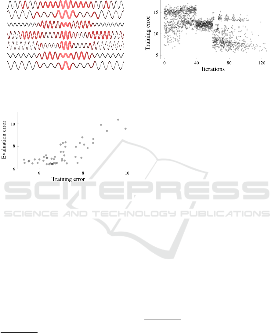
Figure 4: A few sample sequences from the evaluation
data, with anomaly scores taken from a method with a
low evaluation error (6.4), corresponding to α
′
win
(30,10),
β
′
local
(100), η
win
(30,5), θ
vec
(30), ζ
kNN
(δ
DTW
,1), and
κ
mean
.
Figure 5: Average training vs evaluation error for 50 solver
runs, with 10 training items and 100 and evaluation items.
date values for each parameter) and a set T ⊂ P (C×
[0,1]) of training data. It uses the Euclidean distance
(with a prior rescaling of the anomaly scores to [0,1])
as e
′
.
The solver employs a na¨ıve, two-phase optimiza-
tion heuristic: In the first phase, the solver evalu-
ates all valid combinations of sub-methods. For each
such combination, it randomly samples the parameter
space (the product of the sets of sub-method param-
eter values) a fixed number of times, and evaluates
each resulting method on the training data.
In the second phase, the solver uses hill climb-
ing to calibrate the sub-method combination that pro-
duced the lowest error in the first phase
9
.
We applied this solver to a procedurally generated
data set consisting of real-valued sequences with col-
lective contextual anomalies
10
, as illustrated in Fig-
9
Specifically, by starting at the point (out of those sam-
pled) with the smallest error, and iteratively—until a (local)
minimum is found—evaluating all adjacent points (chang-
ing one parameter at a time) and moving to the one with the
lowest error.
10
Specifically: 500-element, sinusoidal real-valued se-
quences with an angular frequency ω ∈ U(1,2) and two dis-
tinct amplitudes a
1
,a
2
(where a
1
= 1, and a
2
is U(1.3,1.7)
Figure 6: The training error at each iteration for a set of
solver executions. Each sub-method combination is sam-
pled 20 times before the solver switches to hill climbing.
ure 4.
We used the sub-methods presented in the previ-
ous section
11
and a set of 20 randomly sampled train-
ing items, let the solver take 20 random samples of
each valid sub-method combination, and repeated the
experiment 50 times. The resulting methods were
then evaluated on a set of 100 items.
As seen in Figure 5, a large share of the result-
ing methods seem to perform close to optimally. The
solver occasionally gets stuck in local minima, pro-
ducing poorly performing methods. Considering the
simplistic nature of the solver, this is hardly surpris-
ing, and it is likely that a more sophisticated solver
would have performed better. The per-iteration train-
ing data error for 20 experiments is shown in Figure 6,
and a few solutions produced by one method with a
low evaluation error is shown in Figure 4.
10 CONCLUSIONS
We have introduced an application-agnostic approach
to anomaly detection, in which anomaly detection
methods are treated as formal objects that may be de-
composed and recombined.
We have applied this formalism to sequences,
showing that it may be used to easily express a wide
range of anomaly detection tasks for this type of data.
Finally, we have demonstrated that our approach
may be used to construct application-agnostic soft-
with probability 0.5 and U(0.3,0.7) with probability 0.5),
arranged in a a-b-c-b-a pattern, where the width of the c re-
gion is U(15,30) (rounded so that the amplitude transition
happens at the nearest sign change), and the width of the b
regions is U(80,100) (also rounded).The labels were set to
1 in the anomalous regions and 0 elsewhere.
11
Specifically, α
′
win
(w,s), β
′
local
(m), β
′
novelty
, the trivial
β
′
used for collective anomalies, η
win
(w,s
′
), θ
vec
(w), and
ζ
kNN
(d, k), for s, s
′
in{5,10,. . . , 25}, w ∈ {30,35,. . . , 60},
k ∈ {1,2,. . . ,5}, m ∈ {80,90,... ,130}, d ∈ {d
E
,d
DTW
}
A Formal Approach to Anomaly Detection
325

ware that facilitates implementing and evaluating
methods, and that can be used to automatically find
appropriate methods (given labeled training data and
a set of candidate sub-methods).
Future Work. We foresee several venues for future
work.
First, there are plenty of interesting sub-methods,
transforms, ensemble methods, and non-sequence
types of data (e.g. graphs, spatial data) to which our
formalism could be extended. There is work to be
done both in terms of studying these and in terms of
creating flexible and efficient implementations.
There is also work to be done on efficiently solv-
ing the optimization problem outlined in Section 9;
we have demonstrated that it may solved for simple
tasks, but it remains to be seen if it can be effectively
solved for real-world tasks.
Finally, modifying or extending our formalism
could be valuable. For instance, associating addi-
tional information with sub-methods could enable al-
gorithms that can optimize or approximate the result-
ing methods.
REFERENCES
Abraham, B. and Box, G. E. (1979). Bayesian analysis
of some outlier problems in time series. Biometrika,
66(2):229–236.
Abraham, B. and Chuang, A. (1989). Outlier detection and
time series modeling. Technometrics, 31(2):241–248.
Agyemang, M., Barker, K., and Alhajj, R. (2006). A
comprehensive survey of numeric and symbolic out-
lier mining techniques. Intelligent Data Analysis,
10(6):521–538.
Basu, S. and Meckesheimer, M. (2007). Automatic outlier
detection for time series: an application to sensor data.
Knowledge and Information Systems, 11(2):137–154.
Berndt, D. J. and Clifford, J. (1994). Using dynamic time
warping to find patterns in time series. In KDD work-
shop, volume 10, pages 359–370.
Chandola, V. (2009). Anomaly detection for symbolic se-
quences and time series data. PhD thesis, University
of Minnesota.
Chandola, V., Banerjee, A., and Kumar, V. (2009).
Anomaly detection: A survey. ACM Computing Sur-
veys (CSUR), 41(3):15.
Chandola, V., Banerjee, A., and Kumar, V. (2012).
Anomaly detection for discrete sequences: A survey.
Knowledge and Data Engineering, IEEE Transactions
on, 24(5):823–839.
Chen, Y., Keogh, E., Hu, B., Begum, N., Bag-
nall, A., Mueen, A., and Batista, G. (2014).
The ucr time series classification archive.
www.cs.ucr.edu/˜eamonn/time
series data/. Accessed:
2014-09-13.
Ding, H., Trajcevski, G., Scheuermann, P., Wang, X., and
Keogh, E. (2008). Querying and mining of time series
data: experimental comparison of representations and
distance measures. Proceedings of the VLDB Endow-
ment, 1(2):1542–1552.
Etsy (2015). Etsy Skyline. github.com/etsy/skyline. Ac-
cessed: 2015-02-10.
Fox, A. J. (1972). Outliers in time series. Journal of the
Royal Statistical Society. Series B (Methodological),
pages 350–363.
Fu, A. W.-C., Leung, O. T.-W., Keogh, E., and Lin, J.
(2006). Finding time series discords based on Haar
transform. In Advanced Data Mining and Applica-
tions, pages 31–41. Springer.
Fu, T.-c. (2011). A review on time series data min-
ing. Engineering Applications of Artificial Intelli-
gence, 24(1):164–181.
Galeano, P., Pe˜na, D., and Tsay, R. S. (2006). Outlier de-
tection in multivariate time series by projection pur-
suit. Journal of the American Statistical Association,
101(474):654–669.
Hodge, V. J. and Austin, J. (2004). A survey of outlier de-
tection methodologies. Artificial Intelligence Review,
22(2):85–126.
Keogh, E., Lin, J., and Fu, A. (2005). Hot sax: Efficiently
finding the most unusual time series subsequence. In
Data mining, fifth IEEE international conference on.
Keogh, E., Lin, J., Lee, S.-H., and Van Herle, H. (2007).
Finding the most unusual time series subsequence: al-
gorithms and applications. Knowledge and Informa-
tion Systems, 11(1):1–27.
Lazarevic, A., Ert¨oz, L., Kumar, V., Ozgur, A., and Sri-
vastava, J. (2003). A comparative study of anomaly
detection schemes in network intrusion detection. In
SDM, pages 25–36.
Lin, J., Keogh, E., Wei, L., and Lonardi, S. (2007). Ex-
periencing sax: a novel symbolic representation of
time series. Data Mining and Knowledge Discovery,
15(2):107–144.
Ma, J. and Perkins, S. (2003). Online novelty detection on
temporal sequences. In Proceedings of the ninth ACM
SIGKDD international conference on Knowledge dis-
covery and data mining, pages 613–618.
Markou, M. and Singh, S. (2003a). Novelty detection: a re-
view, part 1: statistical approaches. Signal processing,
83(12):2481–2497.
Markou, M. and Singh, S. (2003b). Novelty detection: a re-
view—part 2:: neural network based approaches. Sig-
nal processing, 83(12):2499–2521.
Phua, C., Lee, V., Smith, K., and Gayler, R. (2010). A
comprehensive survey of data mining-based fraud de-
tection research. arXiv preprint arXiv:1009.6119.
Tsay, R. S., Pe˜na, D., and Pankratz, A. E. (2000). Outliers in
multivariate time series. Biometrika, 87(4):789–804.
Twitter (2015). AnomalyDetection R Package.
github.com/twitter/anomalydetection. Accessed:
2015-02-10.
ICPRAM 2016 - International Conference on Pattern Recognition Applications and Methods
326
