
Regularization Terms for Motion Estimation
Links with Spatial Correlations
Yann Lepoittevin and Isabelle Herlin
INRIA, Institut National de Recherche en Informatique et Automatique, Le Chesnay, France
Keywords:
Covariance Matrix, Image Assimilation, Motion, Tikhonov Regularization.
Abstract:
Motion estimation from image data has been widely studied in the literature. Due to the aperture problem,
one equation with two unknowns, a Tikhonov regularization is usually applied, which constrains the estimated
motion field. The paper demonstrates that the use of regularization functions is equivalent to the definition
of correlations between pixels and the formulation of the corresponding correlation matrices is given. This
equivalence allows to better understand the impact of the regularization with a display of the correlation values
as images. Such equivalence is of major interest in the context of image assimilation as these methods are
based on the minimization of errors that are correlated on the space-time domain. It also allows to characterize
the role of the errors during the assimilation process.
1 INTRODUCTION
As well known and extensively discussed in the lit-
erature of image processing, motion estimation from
image data is an ill-posed problem, according to the
Hadamard definition (Hadamard, 1923). This comes
from the fact that only one equation is available, the
optical flow equation (Horn and Schunk, 1981), for
estimating two unknown variables, the horizontal and
vertical components, u and v, of the motion vector w.
Smoothing of the motion field, according to the
design of Tikhonov regularization terms (Tikhonov,
1963), is often used in the literature in order to get
a unique solution, as seen for instance in the papers
(Nagel and Enkelmann, 1986), (Nielsen et al., 1994)
or more recently in (Werlberger et al., 2010). A huge
literature is available on the subject. Survey papers on
optical flow have been published, as for instance (Sun
et al., 2010) and (Fortun et al., 2015).
An alternative to the Tikhonov regularization
comes from the use of image assimilation methods,
which include, in the estimation process, the available
heuristics on the temporal evolution of the observed
system. The reader can refer, for example, to the
methods presented in (Papadakis et al., 2010), (Ridal
et al., 2011) or in (B´er´eziat and Herlin, 2011). In the
last few years, a number of such techniques were de-
fined for various contexts of motion estimation from
image sequences.
The data assimilation approach used in the pa-
per is a 4D-Var method, based on the control the-
ory. The foundational paper of Le Dimet and Tala-
grand (Le Dimet and Talagrand, 1986) describes the
computation of the solution of a 4D-Var data assimi-
lation algorithm, thanks to the adjoint method.
The 4D-Var image assimilation, which is applied
in the paper, works as follows. Starting from a back-
ground value, a simulation model is integrated in
time, producing a state vector value at each time step
of the studied temporal interval. At each acquisition
date, the state vector is compared to characteristics
calculated on the image observations. For minimizing
their difference on the whole temporal interval, the
data assimilation method computes an optimal initial
value, named the analysis vector. The whole tempo-
ral trajectory is then obtained by integrating the model
from that analysis value. Section 2 describes the main
mathematical components of the 4D-Var framework.
In order to estimate motion, the 4D-Var approach
defines a cost function J, which is minimized for com-
puting the result. This cost function is depending on
the discrepancy between the state vector and the im-
age data, or image characteristics, at acquisition dates.
Regularization terms are often added to that cost func-
tion, as described by B´er´eziat et al. in (B´er´eziat and
Herlin, 2011), in order to determine the vectorial sub-
space on which motion is estimated. These regu-
larization terms ensure that, during the minimization
process, the motion field keeps the chosen regularity
properties, which are based on the available knowl-
458
Lepoittevin, Y. and Herlin, I.
Regularization Terms for Motion Estimation - Links with Spatial Correlations.
DOI: 10.5220/0005712104560464
In Proceedings of the 11th Joint Conference on Computer Vision, Imaging and Computer Graphics Theory and Applications (VISIGRAPP 2016) - Volume 3: VISAPP, pages 458-466
ISBN: 978-989-758-175-5
Copyright
c
2016 by SCITEPRESS – Science and Technology Publications, Lda. All rights reserved

edge of the observed system.
Three types of regularization are analyzed in the
paper and given in Section 2, simultaneously with a
discussion of their impact on the estimated motion
field. They concern the gradient of motion, its diver-
gence and its norm.
The core of the paper concerns an extensive dis-
cussion on the interpretation of these three regulariza-
tion terms as correlations between pixels of the image
domain. Some related work has been done, for in-
stance, by Dean S. Oliver in (Oliver, 1998), where
the regularization terms are associated to the inverse
of a covariance matrix. Section 3 demonstrates, in the
context of 4D-Var image assimilation, that the estima-
tion result obtained with the regularization terms and
no correlation between pixels is exactly the same than
the one obtained with specific correlations. The cor-
relation matrices corresponding to the three types of
regularization, on the gradient of motion, on its diver-
gence and on its norm, will be given and discussed.
The equivalence between regularization and correla-
tion allows to visualize their joint impact on the esti-
mation and to get insights on the choice of the param-
eters values, which weight these regularization terms.
The displays of correlation matrices are also given in
Section 3.
1.1 Notations
In the remaining of this introduction, the main math-
ematical notations used in the paper are given.
• Let Ω be an open subset of IR
2
. Ω is the image
domain on which motion is estimated.
• Let [0, T] be a closed subset of IR, corresponding
to the time interval on which image acquisitions
are available.
• Ω
T
= Ω × [0, T] defines the studied spatio-
temporal interval, on which image assimilation is
applied.
• A point of the image domain Ω is denoted by:
x =
x y
T
(1)
with x and y corresponding respectively to the ab-
scissa and the ordinate, in a Cartesian system de-
fined on Ω.
• Let w denote the motion function, defined on Ω
T
,
such that:
w(x, t) =
u(x, t) v(x, t)
T
(2)
with u and v quantifying respectively the values of
motion along the abscissa and the ordinate.
• An image function I is defined on Ω
T
, with the
same physical properties as the image acquisi-
tions. I is supposed to be transported by the mo-
tion function w. Consequently, this image func-
tion corresponds to a passive tracer of the motion
function.
• Let introduce the notation X, denoting the state
vector of the observed system, dependingon x and
t and defined on Ω
T
by:
X(x, t) =
w(x, t) I(x, t)
T
(3)
• The image function I and both components, u and
v, of the motion field w are defined on Ω
T
. For
sake of simplicity, we denote u the space-time
function, u(t) the field at date t and u(x, t) the
value at pixel x and date t of the image domain
Ω. The same rule is applied for all functions de-
fined on Ω
T
.
• Data assimilation methods are functioning by
comparing a model output with observed values
of the studied system. The observation vector Y
is defined on Ω
T
. Its value at date t and point x is
Y(x, t). Its components correspond to image ac-
quisitions or to image features computed on these
acquisitions. They are denoted by using the su-
perscript ·
O
. For instance, the image acquisition
is denoted I
O
. I
O
(x, t) is the value at date t and
point x.
• When describing a data assimilation method, pro-
jection operators are needed that are denoted IP.
For instance, IP
w
is the projection from the space
of the state vector on the space of the motion
fields.
• When defining the formulation of the optimal esti-
mation, error terms, denoted ε, are needed. These
error terms will be considered as Gaussian and
zero-mean. They are therefore described by a co-
variance function. The covariance function of the
error term denoted ε
B
is B.
• For describing the implementation, the image do-
main Ω is discretized but is still denoted with the
same symbol, for sake of simplicity. In the same
spirit, x denotes either the point of the continuous
domain or the pixel of the discrete domain, with
indexes i and j. The same rule is applied for all
quantities, X, Y, u, v, I, ...
The image domain is composed of N
Ω
pixels.
The state vector X has N
X
= 3N
Ω
components, as
it includes the value of motion and image for each
pixel.
The vector u has N
Ω
components, which are the
values of u at all pixels. The same goes for v and
I.
Regularization Terms for Motion Estimation - Links with Spatial Correlations
459

The discrete observation vector Y has N
Y
compo-
nents.
The notation t of the continuous time variable is
also kept for the discrete time index.
2 MOTION ESTIMATION AND
REGULARIZATION TERMS
This section summarizes the issue of motion estima-
tion, based on data assimilation methods, as described
for instance in (B´er´eziat and Herlin, 2011).
The first element to be defined is the Image Model,
expressing the heuristics on the observed system and
on the image acquisitions. The design of this Image
Model depends on the duration of the studied tempo-
ral interval. On a short term, the motion field is usu-
ally considered as stationary, which is mathematically
written as:
∂w
∂t
= 0 (4)
Such simple evolution law has a great potential for
operational applications, as no temporal integration
of the motion field is required: w(t) = w(0) for each
value of t. On a longer duration, this assumption is no
more valid and has to be released. In this paper, mo-
tion is considered as advected by itself. This is written
as:
∂w
∂t
+ (w· ∇)w = 0 (5)
It corresponds to the Lagrangian conservation of mo-
tion on the whole trajectory:
dw
dt
(x, t) = 0 (6)
Expressing the motion field w with its two compo-
nents u and v,
w =
u v
T
, (7)
allows to decompose Equation (5) with two partial
differential equations:
∂u
∂t
+ u
∂u
∂x
+ v
∂u
∂y
= 0 (8)
∂v
∂t
+ u
∂v
∂x
+ v
∂v
∂y
= 0 (9)
Considering the hypothesis that the image bright-
ness is a physical property, which is preserved over
time accordingly to the displacement of objects on the
image domain, leads to:
I(x, t) = I(x+ δx, t + δt) (10)
Assuming that the displacement δx and the time inter-
val δt are small, Equation (10) is developed, accord-
ingly to Taylor series, into:
I(x+ δx, t + δt) = I(x, t) + δx
∂I
∂x
+ δt
∂I
∂t
+ . . . (11)
From Equations (10) and (11), it comes:
∂I
∂t
≈ −
δx
δt
∂I
∂x
(12)
Therefore, the image brightness is considered trans-
ported by the motion field, which conducts to the op-
tical flow equation:
∂I
∂t
+ w· ∇I = 0 (13)
The image assimilation approach, which estimates
X with a 4D-Var algorithm, is then based on the fol-
lowing system of three equations:
∂X
∂t
(x, t) + IM(X)(x, t) = 0 (14)
X(x, 0) = X
(b)
(x) + ε
B
(x) (15)
IH(X, Y)(x, t) = ε
R
(x, t) (16)
Equation (14) is the partial differential equation
ruling the temporal evolution of X(x, t). This equation
comes either from Equations (4, 13) or (5, 13). The
value X(x, t) is determined, for any date t, from the
initial value X(x, 0) and the temporal integration of
the model IM.
Equation (15) expresses the a priori knowledge,
named the background value and denoted X
(b)
(x),
that is available on the state vector at initial date 0.
An error term, ε
B
(x), is added in order to express
the uncertainty on this a priori knowledge. This error
term is supposed to be Gaussian and zero-mean, with
the covariance function denoted B. The choice of the
background value is depending on the experiment that
is conducted and is described together with the stud-
ied images. However, as the objective is to estimate
the motion field from the image data, no constraint
will be applied for ensuring that the result stay close
to the background value of motion. This background
motion field is only used as a starting point for the it-
erative minimization process. The background of the
image function I is generally taken as the first acquisi-
tion of the sequence. Equation (15) is then equivalent
to:
I(x, 0) − I
(b)
(x) = ε
B
(x) (17)
where the symbol ε
B
(x) is now used to indicate the
zero-mean Gaussian error on the image component,
associated to its covariance function B. We assume
that the image error is uncorrelated in space. There-
fore B is a diagonal matrix, whose diagonal values are
denoted σ
2
.
VISAPP 2016 - International Conference on Computer Vision Theory and Applications
460

Equation (16) is the observation equation that
links the values of the image acquisitions to the state
vector, at each date of the studied interval. In the
paper, the observation vector Y(x, t) is equal to the
observed image I
O
(x, t) and IH allows to compare
the image function I(x, t) to the image acquisitions
I
O
(x, t). The operator IH is then defined by:
IH(X, Y)(x, t) = I(x, t) − I
O
(x, t) (18)
The observation equation, Equation (16), then
rewrites:
I(x, t)− I
O
(x, t) = ε
R
(x, t) (19)
The discrepancy between the image function I(x, t)
and the acquisition I
O
(x, t) is described by the error
ε
R
(x, t) on the image component. ε
R
(x, t) represents
both the acquisition and representativity errors. This
error term is also supposed Gaussian, zero-mean and
uncorrelated with ε
B
. In the paper, the covariance
function R, associated to ε
R
(x, t), considers no covari-
ance between two locations. Therefore R is a diagonal
matrix, whose diagonal values are also taken equal to
σ
2
.
Solving System (14, 17, 19) is equivalent with the
minimization of the error terms ε
R
and ε
B
. This is ob-
tained by designing a cost function J, depending on
the control variable X(0), with the following formu-
lation (where the space variable x is suppressed for
sake of clarity):
J(X(0)) =
Z
Ω
I(0) − I
(b)
B(x)
−1
I(0) − I
(b)
+
Z
Ω
T
I(t) − I
O
R
−1
I(t) − I
O
(20)
Three regularization terms R
1
, R
2
and R
3
are
added to the cost function of Equation (20). This new
cost function, still denoted J, is minimized during the
data assimilation process, which estimates X(0) and
its motion component.
The first regularization term, named R
1
, acts on
the norm of the gradient of the motion field. It is de-
signed as follows:
R
1
(X(0)) = α
Z
Ω
||∇(IP
w
(X(x, 0)))||
2
dx (21)
or equivalently:
R
1
(X(0)) = α
Z
Ω
||∇w(x, 0)||
2
dx (22)
R
1
ensures the spatial smoothness of the estimation.
It is weighted by the parameter α.
When working on the issue of sea surface circula-
tion, the estimated motion field should be divergence
free, due to the incompressibility property. In other
applications, even if the divergence is non null, its
value should be small as aliasing effects could appear,
during the temporal integration of the image model, if
the divergence is high. A second regularization term
R
2
, acting on the divergence, is then added to the cost
function J:
R
2
(X(0)) = β
Z
Ω
[div(IP
w
(X(x, 0)))]
2
dx (23)
or equivalently:
R
2
(X(0)) = β
Z
Ω
[div(w(x, 0))]
2
dx (24)
where:
div(w(x, 0)) =
∂u
∂x
(x, 0) +
∂v
∂y
(x, 0) (25)
A regularization term acting on the norm of the
motion field is also included in the function J, in order
to avoid having spurious high values of w. This term
R
3
is defined by:
R
3
(X(0)) = γ
Z
Ω
||IP
w
(X(x, 0))||
2
dx (26)
or equivalently:
R
3
(X(0)) = γ
Z
Ω
||w(x, 0)||
2
dx (27)
Let sum up these three regularization into a global
term R , defined as:
R = R
1
+ R
2
+ R
3
(28)
and depending on the initial value X(0) through its
motion component w(0).
Having defined the regularization terms, the next
section will discuss and illustrate their significance
and action during the estimation process.
3 SIGNIFICANCE OF THE
REGULARIZATION
The regularization terms, which are included in the
cost function are given, with a variational formula-
tion, in Equations (22, 24, 27). Keeping in mind that
w =
u
v
, it is possible to rewrite the formulation of
R
1
Equation (22), as:
R
1
(X(0)) = α
Z
Ω
∂u
∂x
(x, 0)
2
+
∂u
∂y
(x, 0)
2
+
∂v
∂x
(x, 0)
2
+
∂v
∂y
(x, 0)
2
(29)
Regularization Terms for Motion Estimation - Links with Spatial Correlations
461

The formulation of R
2
in Equation (24) is rewritten
as:
R
2
(X(0)) = β
Z
Ω
∂u
∂x
(x, 0) +
∂v
∂y
(x, 0)
2
(30)
Last, R
3
of Equation (27) is equal to:
R
3
(X(0)) = γ
Z
Ω
u(x, 0)
2
+ v(x, 0)
2
(31)
When implementing the method on a discrete the
image domain Ω, the derivatives along x and y are
computed by filters D
x
and D
y
, whose values depend
on the chosen discretization schemes. If the deriva-
tives are, for instance, approximated with a forward
scheme, the filter D
x
is defined by:
D
x
=
0 0 0
0
−1
dx
1
dx
0 0 0
(32)
and the filter D
y
by:
D
y
=
0
1
dy
0
0
−1
dy
0
0 0 0
(33)
The derivative filters being applied on the whole do-
main, let introduce the matrices D
x
and D
y
, which
compute the discrete derivatives at every pixel, re-
spectively along the directions x and y. By defini-
tion, D
x
and D
y
are Toeplitz matrices and their coef-
ficients along descending diagonals are constant. For
instance, D
x
has the value
−1
dx
on its main diagonal and
the value
1
dx
on the first above diagonal:
D
x
=
1
dx
−1 1
−1 1
−1 1
.
.
.
.
.
.
−1 1
−1
(34)
It is then possible to rewrite the discrete formulation
of each regularization term from these notations.
The discrete version of Equation (29) is:
R
1
(X(0)) = α
hD
x
u , D
x
ui + hD
y
u , D
y
ui
+ hD
x
v , D
x
vi + hD
y
v , D
y
vi
(35)
where h f
1
, f
2
i denotes the scalar product of the vec-
tors v
1
and v
2
. Equation (30) leads to:
R
2
(X(0)) = βhD
x
u+ D
y
v , D
x
u+ D
y
vi (36)
Equation (31) is discretized by:
R
3
(X(0)) = γ
hu , ui + hv , vi
(37)
Let introduce the vector
u
v
of size 2N
Ω
in the
previous scalar products. Let also use the fact that
D
x
and D
y
being matrices with real coefficients, their
adjoint is equal to their transpose. Let furthermore
use the bilinearity of the scalar product. These three
points lead to rewrite the discrete formulation of R
1
in Equation (35) as:
u
v
, α
K 0
0 K
u
v
(38)
with K being defined by:
K = D
T
x
D
x
+ D
T
y
D
y
(39)
The discrete formulation of R
2
, in Equation (36),
leads to:
u
v
, β
D
T
x
D
x
D
T
x
D
y
D
T
y
D
x
D
T
y
D
y
u
v
(40)
Last, the formulation of R
3
, in Equation (37), be-
comes:
u
v
, γ
II 0
0 II
u
v
(41)
where II is the identity matrix.
Let denote C
1
the matrix involved in the computa-
tion of R
1
, Equation (38):
C
1
= α
K 0
0 K
(42)
Let denote C
2
the matrix involved in Equation (40):
C
2
= β
D
T
x
D
x
D
T
x
D
y
D
T
y
D
x
D
T
y
D
y
(43)
Let denote C
3
the matrix obtained in Equation (41):
C
3
= γ
II 0
0 II
(44)
Last, let define the matrix C:
C = C
1
+C
2
+C
3
(45)
=
αK + βD
T
x
D
x
+ γII βD
T
x
D
y
βD
T
y
D
x
αK + βD
T
y
D
y
+ γII
The definition of C leads to the following equality for
the regularization term involved in the cost function:
R (X(0)) =
u
v
, C
u
v
(46)
As R
1
(in Equation (22)), R
2
(in Equation (24))
and R
3
(in qEquation (27)) are positive or null, as
long as α, β and γ are positive, the regularization
value expressed in Equation (28) is also positive or
null. Moreover, R (X(0)) is null if and only if w(0)
is null. As both formulation of the regularization,
VISAPP 2016 - International Conference on Computer Vision Theory and Applications
462

Equations (28) and (46) are equivalent, the matrix C
is symmetric definite positive and can be considered
as the inverse of a covariance matrix B
R
.
It comes that the two following formulations of
the discrete cost function (where the space and time
indexes are suppressed for sake of clarity) are equiva-
lent:
D
I(0) − I
(b)
, B
−1
I(0) − I
(b)
E
+
∑
[0,T]
I − I
O
, R
−1
I − I
O
+ R (X(0)) (47)
and:
D
X(0) − X
(b)
, B
−1
R
X(0) − X
(b)
E
+
∑
[0,T]
I − I
O
, R
−1
I − I
O
(48)
where the new covariance matrix B
R
verifies:
B
−1
R
=
C 0
0 B
−1
(49)
It should be noted that, in Equation (47), only the im-
age component I
(b)
of X
(b)
is involved and is chosen
equal to the first image acquisition I
O
(0). On another
hand, in Equation (48), the whole background vector
is involved and defined by:
X
(b)
=
0
0
I(0)
(50)
where the image component is the same and the mo-
tion component is given a null value, which provides
the heuristic of smoothness for the motion field. The
error covariance matrix B of the image background
keeps the same value from Equation (47) to Equa-
tion (49).
This concludes the demonstration that the use of
regularization terms is equivalent to the use of a non
diagonal covariance matrix B
R
in the cost function
minimized for estimating motion.
When implementing the image assimilation
method, the state vector X(0) is composed of the three
components u(0), v(0), and I(0). Each of these com-
ponents is defined on the discrete image domain Ω,
composed of N
Ω
pixels. Therefore, X(0) has 3N
Ω
components. The size of the covariance matrix B
is equal to the square of the size of the state vec-
tor. This would lead to unaffordable memory costs
if one wants to store the whole matrix. For instance,
for a 100× 100 pixels image, this leads to a 54 giga-
bytes matrix. However, the inverse matrix designed
in Equation (49) is sparse and contains a high number
of zero values. A sparse storage of this covariance
matrix is feasible, but would lead to high computa-
tional costs when performing the matrix inversion or
the product of the matrix by a vector, for instance in
Equation (48). Therefore, the solution of minimizing
Equation (48) by designing the covariance matrix B
R
and inverting it is not considered for the operational
use of the image assimilation method.
Let however remark that B
R
is not required for
computing the cost function with Equation (48) but
only its inverse B
−1
R
is. As the blocks included in
B
−1
R
are Toeplitz matrices, the best way to compute
the value of the cost function J with Equation (48) is
to consider each block of B
−1
R
as a discrete filter. Let
first remark that the filter associated to B
−1
is defined
by:
B
−1
=
0 0 0
0
1
σ
2
0
0 0 0
(51)
For further illustrating the discussion, let consider that
the derivatives are computed with forward schemes,
which are determined by the following convolution
filters:
Dx =
0 0 0
0
−1
dx
1
dx
0 0 0
, Dy =
0
1
dy
0
0
−1
dy
0
0 0 0
(52)
Let denote B
−1
R
i, j
the bloc on the i
th
line and j
th
column
of B
−1
R
, as it is written in Equation (49), considering
the definition of C given by Equations (45) and (39).
Let denote B
−1
R
i,j
the corresponding convolution filter.
Using the mathematical rules for addition and com-
position of filters, it comes:
B
−1
R
1,1
=
0 −α 0
−(α+ β) L
1
−(α+ β)
0 −α 0
(53)
where:
L
1
= 2
α+ β
dx
2
+
β
dy
2
+ γ (54)
B
−1
R
2, 2
=
0 −(α+ β) 0
−α L
2
−α
0 −(α+ β) 0
(55)
where:
L
2
= 2
β
dx
2
+
α+ β
dy
2
+ γ (56)
Regularization Terms for Motion Estimation - Links with Spatial Correlations
463
B
−1
R
1,2
=
β
dxdy
−β
dxdy
0
−β
dxdy
β
dxdy
0
0 0 0
(57)
B
−1
R
2, 1
=
0 0 0
0
β
dxdy
−β
dxdy
0
−β
dxdy
β
dxdy
(58)
The use of B
−1
R
during the computation of J with
Equation (48) is replaced by the use of the four pre-
vious filters. The design of this non diagonal ma-
trix B
R
is equivalent, as demonstrated above, to ap-
ply the regularization R to the state vector. However,
the covariance method has the advantage, compared
to the regularization method, that the derivatives of
the regularization functions defined by Equations (22,
24, 27) are no more required during the minimiza-
tion. Moreover, the filters included in the matrix B
−1
R
,
Equations (49, 45, 39), are applied both in the for-
ward integration, computing the cost function J of
Equation (48), and in the backward integration, which
computes the gradient
dJ
dX(0)
:
dJ
dX(0)
= 2B
−1
R
X(0) − X
(b)
+ λ(0) (59)
Studying the values of the covariance matrix B
R
,
corresponding to the values of the coefficients α, β
and γ is a tool for better understanding the impact of
the regularization R on the estimation. For doing this,
it is first required to invert the matrix B
−1
R
, defined in
Equations (49, 45, 39), in order to obtain the covari-
ance matrix B
R
. This can not be done in operational
use, due to the large size of the involved state vectors
(3 times the size of the image domain). Moreover, it
has no interest apart having a complete knowledge of
the links imposed between variables of the state vec-
tor and between pixels of the spatial domain. How-
ever, when designing an operational use of motion
estimation, this allows visualizing and understanding
how the regularization terms act on the estimation re-
sults. This can be applied, during a learning phase for
calibrating the operational use, on small sub-windows
on the whole image domain as explained in the fol-
lowing.
For being able to easily compute the inverse of the
matrix B
−1
R
, we consider a small size sub-image of
35× 35 pixels. One can extract the x
th
line of the co-
variance matrix. It corresponds to the covariance val-
ues of that pixel x with all other pixels of the domain.
In the following, we focus on the visualization of the
covariances in B
R
11
, as they involve the three regular-
ization terms and the three parameters α, β and γ as
visible in Equations (53) and (54). B
R
22
is a rotated
version of B
R
11
and would lead to a redundant visu-
alization. B
R
12
and B
R
21
are only depending on the
term R
2
and on the parameter β (see Equation (55)
and (56)). Their visualization would not allow to im-
prove the understanding of the joint effect of the three
regularization terms.
The term R
3
, regularizing the norm of the motion
field with the parameter γ, acts on the individual vari-
ance and does not add any correlation between pixels.
Varying the two terms R
1
, regularizing the gradient
norm of w with the parameter α, and R
2
, regularizing
the divergence of w with the parameter β, allows to
display the covariance between a reference point and
the rest of the domain. The state vector is composed
of the three fields corresponding to the values of u, v
and I at all locations. The covariance matrix associ-
ated to each field may be displayed as an image.
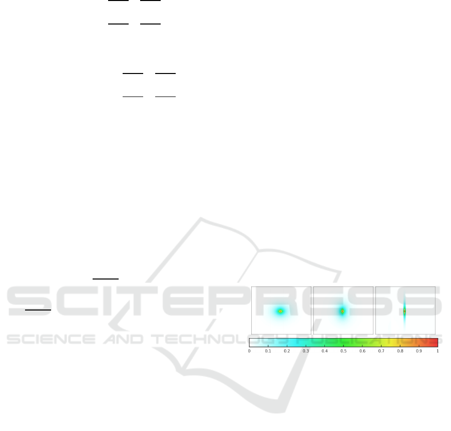
Figure 1 gives the covariance of the component u
of pixel (17, 17) with the rest of the sub-image. On the
left, the coefficient of R
1
is preponderant. In the mid-
dle, R
1
and R
2
have the same importance in the com-
putation. On the right, R
2
is preponderant. It can be
Figure 1: Covariance values associated to the central point
(red pixel); when R
1
is preponderant (on the left); when R
1
and R
2
are of same weight (in the middle); and when R
2
is
preponderant (on the right).
seen that R
1
mimics an homogeneous diffusion pro-
cess. On another hand, R
2
favors specific directions
for creating vortices and limiting the divergenceof the
motion field.
The range of the covariance values is parametrized
by the values of α and β. This is, first, illustrated on
Figure 2, which displays the covariance values asso-
ciated to the regularization term R
1
, according to a
small α, on the left, and a higher one, on the right.
Similarly, Figure 3 shows the covariance values as-
sociated to the regularization term R
2
. On the left
image, a small value of β is used, whereas the right
image shows the covariance values for a higher β.
It can be seen, by analyzing Figure 2 and Figure 3,
that the region of high covariance increases with the
value of the regularization parameters α and β. Dis-
playing a number of such images should help, for a
given, application, to define the parameters values ac-
VISAPP 2016 - International Conference on Computer Vision Theory and Applications
464
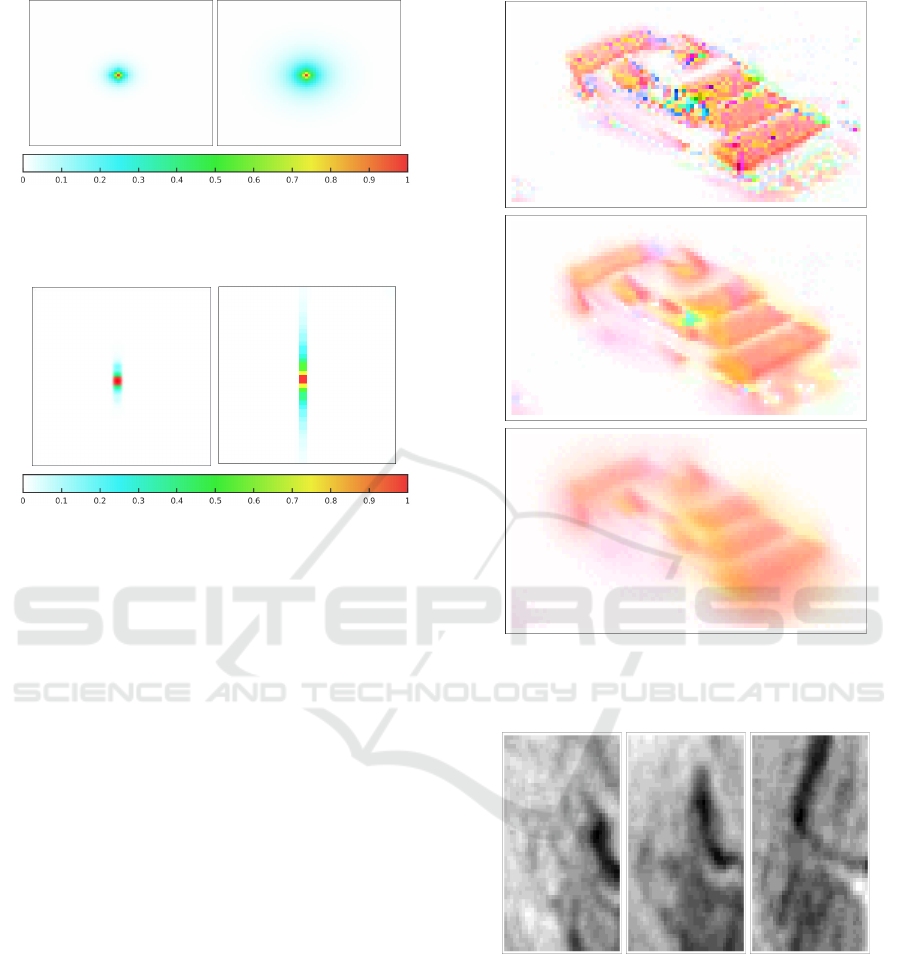
Figure 2: Covariance values associated to the central point
(red pixel) for R
1
only; with a small α (on the left) and a
higher one (on the right).
Figure 3: Covariance values associated to the central point
(red pixel) for R
2
only; with a small β (on the left) and a
higher one (on the right).
cording to the size of the structures to be found on the
images.
For visualizing the impact of the parameters on the
estimation, several motion results are given. On Fig-
ure 4, the estimation is computed on traffic data from
the database KOGS/IAKS of the Karlsruhe Univer-
sity (Nagel, 1995). Motion is displayed with the color
code of the Middlebury data base described by Baker
et al. (Baker et al., 2011). The top image displays
the result obtained with only R
3
. It can be seen that
the motion field is irregular even if its whole shape is
overallwell recovered. The second image displays the
estimation result when adding R
1
, with a small value
of α (this corresponds to the left image of Figure 2).
The estimation is smoother than the one on the top
image, but irregularities remain. The bottom image is
obtained with a large α value (this corresponds to the
right image of Figure 2). The estimation is smooth
without any irregularities.
A sequence of Sea Surface Temperature (SST) is
processed as another illustration of the impact on the
estimation of different parametrizations. Some im-
ages of the sequence are displayed on Figure 5. Result
are shown on Figure 6, where the estimation is either
obtained with R
1
and R
3
or R
2
and R
3
. It can bee
seen, from the left image of Figure 6, that R
1
tends
to favor smooth and homogene motion fields. In the
contrary, as seen from the right image of Figure 6, R
2
Figure 4: From top to bottom: Motion result with R
3
only;
R
3
and R
1
and a small value of α; R
3
and R
1
and a high
value of α.
Figure 5: Sequence of Sea Surface Temperature images.
favors gyral structures to explain the temporal evolu-
tion of the gray level values.
4 CONCLUSIONS
The paper discusses the mathematical links between
the Tikhonov regularization terms and the spatial co-
variances applied between pixels. The application
concerns the issue of motion estimation, which is
Regularization Terms for Motion Estimation - Links with Spatial Correlations
465
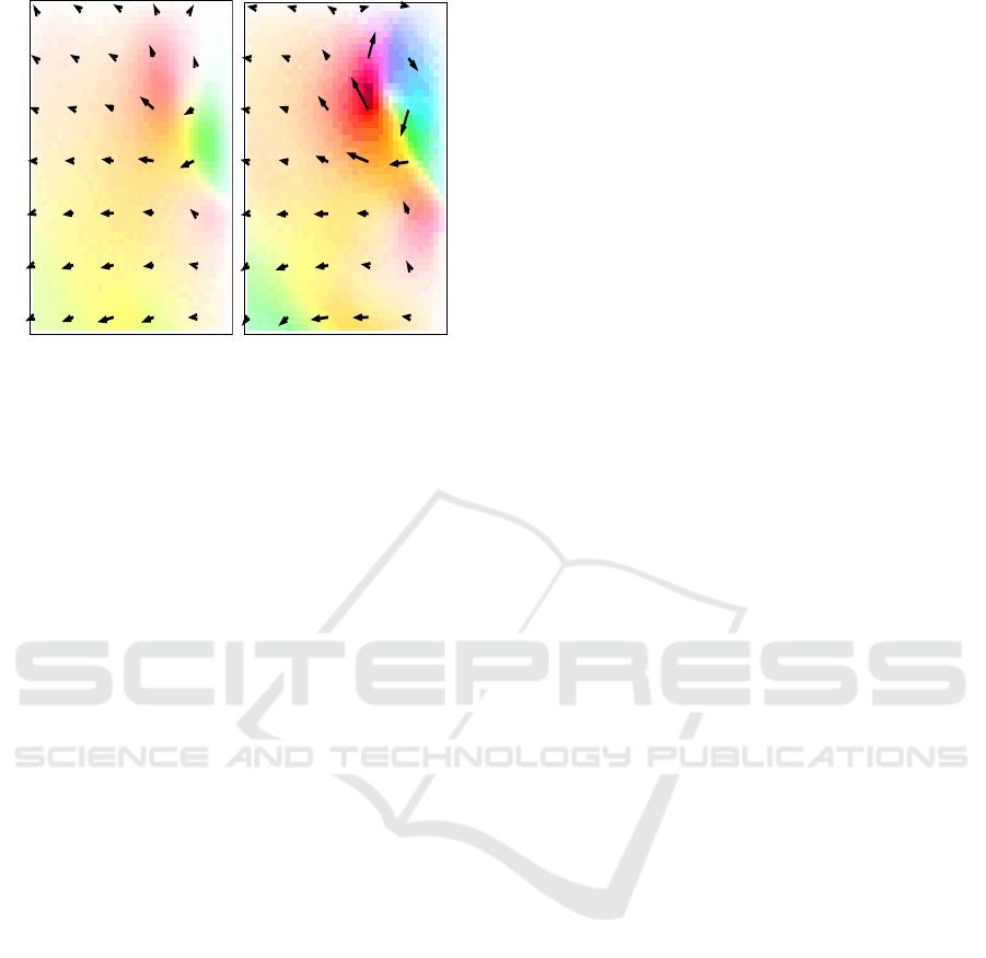
Figure 6: Estimation results obtained on the SST sequence.
Left: Motion result with R
1
and R
3
. Right: Motion result
with R
2
and R
3
.
an ill-posed problem that is often solved by adding
regularization terms in a cost function. In the pa-
per, the framework of motion estimation relies on im-
age assimilation, which also implies to model the co-
variances between pixels, variables and dates. The
major result of that research comes from the dis-
play of the regularization terms as images of corre-
lation values. Analyzing these display regarding the
parametrization of the regularization, enables to visu-
alize the region of high covariance of the regulariza-
tion and allows to objectively determine the values of
the weighting coefficients according to image prop-
erties. The perspectives concern the design and inter-
pretation of regularization terms, which are suitable to
model the structures displayed on image sequences.
ACKNOWLEDGEMENTS
This research has been partially funded by the DGA.
REFERENCES
Baker, S., Scharstein, D., Lewis, J. P., Roth, S., Black, M. J.,
and Szeliski, R. (2011). A database and evaluation
methodology for optical flow. International Journal
on Computer Vision, 92(1):1–31.
B´er´eziat, D. and Herlin, I. (2011). Solving ill-posed image
processing problems using data assimilation. Numer-
ical Algorithms, 56(2):219–252.
Fortun, D., Bouthemy, P., and Kervrann, C. (2015). Optical
flow modeling and computation: A survey. Computer
Vision and Image Understanding, 134:1 – 21.
Hadamard, J. (1923). Lecture on Cauchy’s Problem in Lin-
ear Partial Differential Equations. Yale University
Press, New Haven.
Horn, B. and Schunk, B. (1981). Determining optical flow.
Artificial Intelligence, 17:185–203.
Le Dimet, F. and Talagrand, O. (1986). Variational algo-
rithms for analysis and assimilation of meteorological
observations: theoretical aspects. Tellus Series A : Dy-
namic meteorology and oceanography, 38(2):97–110.
Nagel, H.-H. (1995). Nibelungen-platz. www.ira.uka.de.
Nagel, H. H. and Enkelmann, W. (1986). An investi-
gation of smoothness constraints for the estimation
of displacement vector fields from image sequences.
Pattern Analysis and Machine Intelligence, PAMI-
8(5):565–593.
Nielsen, M., Florack, L., and Deriche, R. (1994). Regular-
isation and scale space. Technical Report RR 2352,
INRIA.
Oliver, D. (1998). Calculation of the inverse of the covari-
ance. Mathematical Geology, 30(7):911–933.
Papadakis, N., M´emin, E., Cuzol, A., and Gengembre, N.
(2010). Data assimilation with the weighted ensemble
Kalman filter. Tellus Series A : Dynamic meteorology
and oceanography, 62(5):673–697.
Ridal, M., Lindskog, M., Gustafsson, N., and Haase, G.
(2011). Optimized advection of radar reflectivities.
Atmospheric Research, 100(2–3):213–225.
Sun, D., Roth, S., and Black, M. (2010). Secrets of opti-
cal flow estimation and their principles. In European
Conference on Computer Vision, pages 2432–2439.
Tikhonov, A. N. (1963). Regularization of incorrectly posed
problems. Soviet Mathematics - Doklady, 4:1624–
1627.
Werlberger, M., Pock, T., and Bischof, H. (2010). Motion
estimation with non-local total variation regulariza-
tion. In Conference on Computer Vision and Pattern
Recognition, San Francisco, CA, USA.
VISAPP 2016 - International Conference on Computer Vision Theory and Applications
466
