Stitching Grid-wise Atomic Force Microscope Images

Mathias Vestergaard

, Stefan Bengtson

, Malte Pedersen

, Christian Rankl

and Thomas B. Moeslund

Institute of Media Technology, Aalborg University, Aalborg, Denmark

AFM R&D, Keysight Technologies, San Fransisco, U.S.A.

Keywords:

Atomic Force Microscopy, RANSAC, Template Matching, Image Stitching.

Abstract:

Atomic Force Microscopes (AFM) are able to capture images with a resolution in the nano metre scale. Due to

this high resolution, the covered area per image is relatively small, which can be problematic when surveying

a sample. A system able to stitch AFM images has been developed to solve this problem. The images exhibit

tilt, offset and scanner bow, which are counteracted by subtracting a polynomial from each line. To be able to

stitch the images properly template selection is done by analyzing texture and using a voting scheme. Grids

of 3x3 images have been successfully leveled and stitched.

1 INTRODUCTION

Atomic Force Microscopes (AFM) are able to create

topography images with very high resolution by trac-

ing the surface of a sample, line-by-line with a tiny

probe. The resolution of the AFMs is in nanometer

scale while conventional optical microscopes, in com-

parison, are able to achieve a maximum resolution

of some hundred nanometers. The limited resolution

of optical microscopes is imposed by the way light

diffracts (Eaton and West, 2010). The high resolution

of the AFM images allows for studies of molecules

(Last et al., 2010) and living cells (Johnson, 2011).

However, the improved resolution comes at the

cost of increased capturing time, as tracing the sur-

face of a sample, line-by-line, is a slow process which

can take several minutes. Another drawback is the

decrease in ﬁeld of view, i.e. the area of the sample

contained in a single image. It is therefore not uncom-

mon for the size of the sample to exceed the viewable

area of the AFM and to counteract this, most AFMs

feature a motorized stage which allows them to auto-

matically capture the sample piece-by-piece.

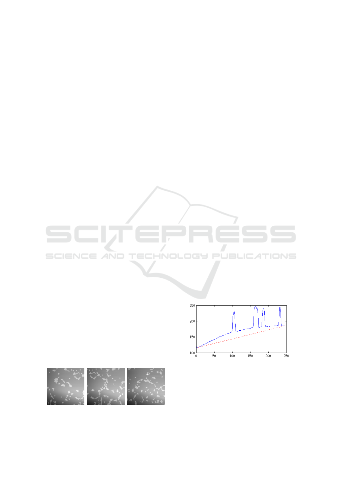
Figure 1: Topography images of bacteria.

The result of this method is a series of images which

provides a fragmented view of the sample as seen in

Figure 1. The three images are overlapping in the hor-

izontal direction, but it is difﬁcult and tedious to work

with this fragmented kind of view. A method to pro-

cess and stitch the images into a single image without

visible seams is therefore wanted.

Because of the high resolution of the AFM even

the smallest ﬂaws will be apparent in the images.

These ﬂaws complicate the stitching process and re-

quire steps to remove potential irregularities. This is

necessary as the ﬁnal image, consisting of several iso-

lated images, should have a uniform background.

Figure 2: A line from one of the bacteria images. The red

line is added to visualize the tilt and scanner bow.

It is difﬁcult to place the sample with enough preci-

sion to ensure a horizontally leveled surface and this

results in a visible tilt, where the images are darker on

one side. An example can be seen in Figure 2, which

illustrates a horizontal line taken from one of the bac-

teria images. The tilt can be seen as the red dashed

112

Vestergaard, M., Bengtson, S., Pedersen, M., Rankl, C. and Moeslund, T.

Stitching Grid-wise Atomic Force Microscope Images.

DOI: 10.5220/0005716501100117

In Proceedings of the 11th Joint Conference on Computer Vision, Imaging and Computer Graphics Theory and Applications (VISIGRAPP 2016) - Volume 3: VISAPP, pages 112-119

ISBN: 978-989-758-175-5

line, which is more or less the same within a speciﬁc

sample, but may vary from one sample to another.

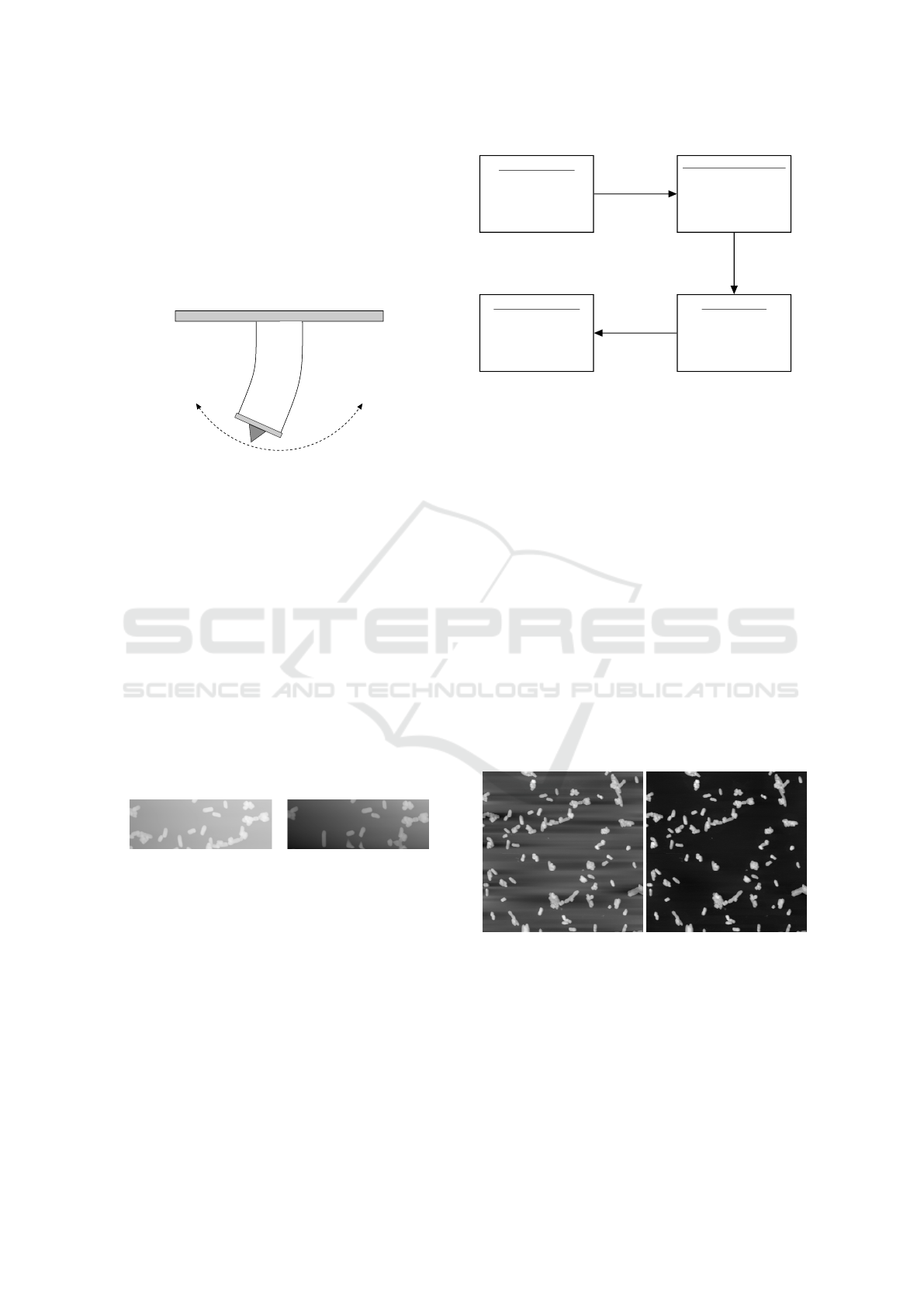
Most AFMs have only one moving part which is a

piezoelectric block that can be placed either beneath

or above the sample. This block is controlled by ap-

plying current to the sides, which results in a move-

ment pattern similar to that of a pendulum, see Fig-

ure 3.

Scanner

tube

Probe

Figure 3: Illustration of the bow is created when a piezo-

electric scanner tube is used to move the probe.

This is especially clear in images where the piezoelec-

tric block is forced to approach its maximum range. A

phenomenon occurs where an even surface appears to

bow and the intensity near the edge of the image is

lower than at the center. This bow can be observed in

Figure 2.

Beside scanner bow and tilt another problem can

occur where some of the objects move or change

shape between the capturing of two adjacent images.

This can happen if the sample consists of living or-

ganisms where movement creates a difﬁculty in ﬁnd-

ing the right blending. The same object can end up

having two different positions, relative to the rest of

the image, if it has moved. In worst case scenarios

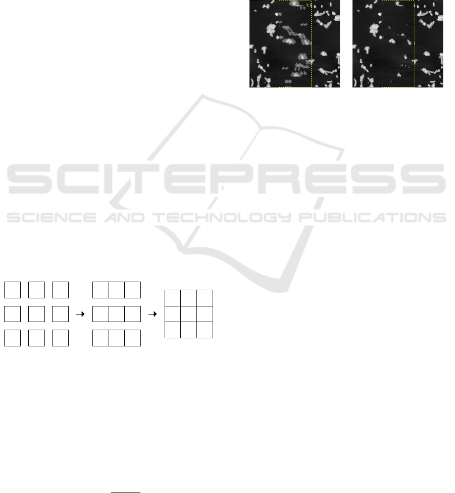
objects are totally missing as seen in Figure 4.

Figure 4: Two subimages showing the same area of a sam-

ple. The subimages are taken from the overlapping part of

two images.

2 APPROACH

The proposed solution contains four modules as illus-

trated in Figure 5. The boxes symbolize the modules

which are: Preprocessing, Feature Extraction, Recog-

nition and Post Processing. Between the modules

are arrows which represent the way of the workﬂow.

These modules will be described in the following sec-

tions.

Preprocessing

Image Leveling

Feature Extraction

Find

Template Positions

Processed Image

Recognition

Template Matching

Template Positions

Post Processing

Translation

and

Stitching

Position of

best match

Figure 5: The overall design of the proposed solution.

2.1 Image Leveling

The objective of the leveling process is to remove

scanner bow, tilt and offset, while preserving the ob-

jects in the images. Traditional image processing

techniques are possible solutions, such as the rolling

ball algorithm (Lundtoft, 2014).

However, this approach does not account for the

characteristics of the artifacts. Namely how they can

be described as 2nd order polynomials acquired in a

line-by-line pattern.

A common method to level AFM images is therefore

to ﬁt and then subtract a polynomial line-by-line

for the entire image (Eaton and West, 2010). When

ﬁtting the polynomial it is important to exclude the

objects to avoid overcompensation which could result

in new artifacts (Figure 6).

(a) Objects not excluded. (b) Objects excluded.

Figure 6: The same image leveled with and without object

exclusion.

Some approaches rely on manual selection of objects

to exclude (Eaton and West, 2010), which is very

labour intensive and not useful when dealing with a

lot of images. Another approach is to use K-means

clustering to identify objects in every line (Pan, 2014)

(Tsaftaris et al., 2008).

Stitching Grid-wise Atomic Force Microscope Images

113

2.1.1 Leveling Algorithm

The developed leveling algorithm expands upon the

idea of line-by-line leveling by introducing a new

way of automatically excluding objects through the

use of RANSAC (Random Sample Consensus) (Fis-

chler and Bolles, 1980). RANSAC is suitable as it

is able to estimate parameters of a given model (in

this case a 1st or 2nd order polynomial) from a data

set (a line from the image) contaminated with outliers

(objects). RANSAC basically works by repeatedly

making guesses at a solution based on n randomly se-

lected initial points, where n is the minimum number

of points required to determine the parameters of the

model. Each solution is then evaluated and compared

against the current best guess, yielding the best guess

as the solution in the end.

RANSAC is therefore non-deterministic and its

success depends on the number of iterations k which

RANSAC is allowed to execute. k can be determined

theoretically based on two assumptions:

The solution is considered decent if:

• All the n initial points are inliers, i.e. part of the

polynomial to be removed.

• The n initial points are not closely grouped to-

gether, which is evident be contemplating e.g. 2nd

order polynomials.

For the sake of simplicity, the number of data points

is divided into n evenly sized intervals and the n

initial points are considered to be appropriately

spaced if each resides in an interval of its own.

Hence, the probability of never reaching a de-

cent solution out of k iterations is given by:

P(bad) = (1 − P(in)

× P(spaced))

(1)

where P(in) is the probability of a point being an

inlier and P(spaced) is the probability of the n

points being appropriately spaced, i.e. P(spaced) =

(1/n)

. The probability of reaching a decent solution

P(decent) out of k iterations must then be given by:

1 − P(decent) = (1 − P(in)

× (1/n)

)

(2)

from where k can be isolated:

k =

log(1 − P(decent))

log(1 − P(in)

× (1/n)

)

(3)

Considering a scenario with 50% outliers, i.e. P(in) =

0.50, and it would take:

k =

log(1 − 0.999)

log(1 − 0.50

× (1/3)

)

≈ 1488 (4)

iterations to ﬁnd a decent solution with a probability

of P(decent) = 99.9% when using n = 3 initial

points, which is sufﬁcient for a 2nd order polynomial.

Another solution could be to divide each line

into n evenly sized intervals and then randomly

choose one point from each interval as the n initial

point. This would reduce the number of iterations k

to:

k =

log(1 − P(decent))

log(1 − P(in)

)

(5)

as it is no longer necessary to check the spacing be-

tween the points, i.e. take P(spaced) into account.

However, this method was found to be inconsis-

tent during tests on real data, as it would repeat-

edly fail at images with un-evenly distributed outliers,

where the majority of outliers would reside in one of

the ﬁxed intervals. The idea of using ﬁxed intervals

was therefore discarded.

2.1.2 Performance Considerations

A runtime test of a generic RANSAC algorithm is

performed to determine whether the k = 1488 from

Equation 4 is realistic. The algorithm is implemented

in C++ and is performed on a laptop with a P8600

@ 2.4GHz CPU. On average (100 repetitions) it

took 0.88 seconds to execute the algorithm. Hence,

it would take 3 minutes and 45 seconds to apply

RANSAC on each horizontal line in a relatively small

image of 256 × 256 pixels, which is not acceptable.

In order to reduce runtime, RANSAC is only

used to exclude objects in the ﬁrst line of the image.

In the following lines, the exclusion of objects is

achieved by ignoring every point x in the line l(x)

which is not within a ﬁxed threshold t from the

polynomial p(x)

latest

found in the previous line. I.e.

only points which fulﬁls

> (p(x)

latest

− l(x))

(6)

are used when ﬁtting the polynomial to be subtracted

in every line, apart from the ﬁrst line where RANSAC

is used.

2.1.3 Final Leveling Algorithm

The ﬁnal leveling algorithm is as follows:

1. Fit a polynomial p(x)

latest

to the ﬁrst line l

in the

AFM image using RANSAC.

2. Find inliers in the next line based on p(x)

latest

and

a ﬁxed threshold t.

3. Fit a polynomial to the found inliers and subtract

the found polynomial from the current line.

VISAPP 2016 - International Conference on Computer Vision Theory and Applications

114

4. Overwrite p(x)

latest

with the polynomial just

found.

5. Repeat step 2-4 until all lines have been processed

in the AFM image.

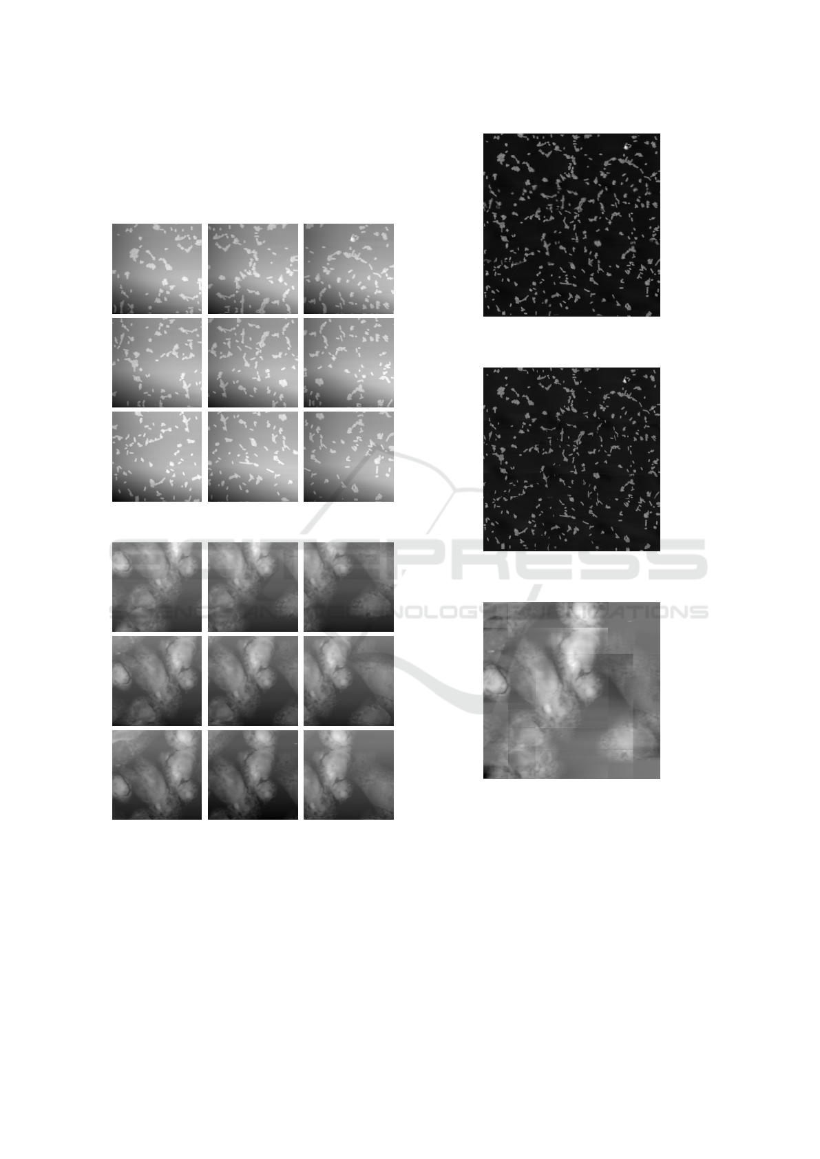
The developed leveling algorithm does well when the

percentage of background is noticeably larger than the

object percentage (Figure 7).

The leveled images will however start to exhibit

an offset in height when the object percentage

approaches or exceeds 50% (Figure 8). This issue

originates in the initial step of the algorithm, where

RANSAC might mistakenly ﬁt a polynomial to the

top of the objects instead of the background.

The above issue can be detected by comparing

the mean of the current line µ

line

with the mean of

the ﬁtted polynomial µ

poly

. The polynomial is then

considered to be ﬁtted correctly if:

line

> µ

poly

(7)

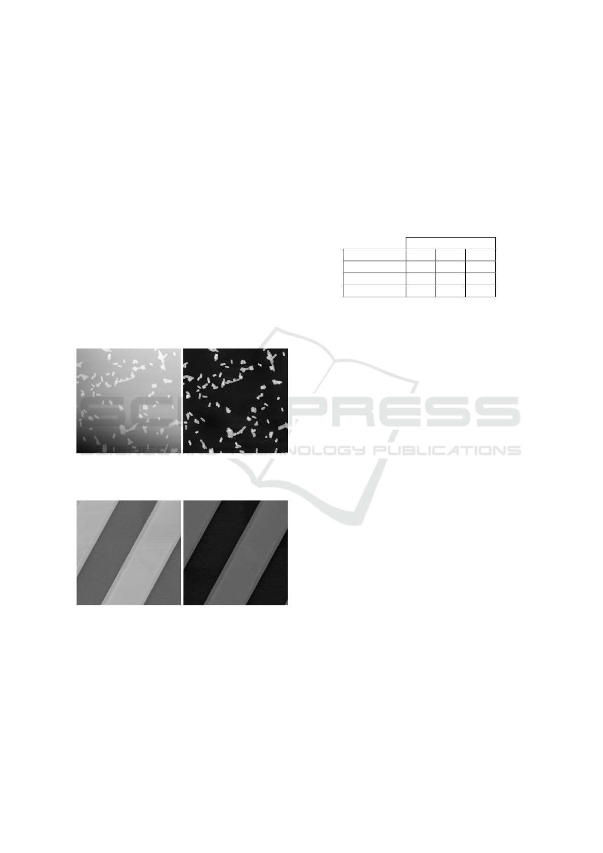
(a) Original image. (b) Leveled image.

Figure 7: Leveling of image with a high background per-

centage.

(a) First image. (b) Second image.

Figure 8: Two adjacent images of SiO

stripes after lev-

eling. The difference in intensity is caused by the height

offset between the images.

The correct polynomial can be found by ﬁtting a poly-

nomial to the outliers, instead of the inliers. This san-

ity check and correction are easily executed at the end

of the developed leveling algorithm.

The average processing time of the developed level-

ing algorithm, including the above sanity check, is

found to be roughly 1 second (see Table 1). This is

deemed acceptable considering the time it takes to

capture each AFM image (several minutes).

The test was performed on a laptop with a P8600

@ 2.4GHz CPU with datasets containing 9 images

each. The bacteria and SiO

stripes datasets contains

images with a resolution of 256 x 256 pixels, while

the bacteria HQ dataset contains images of 512 x 512

pixels. Hence the noticeable difference in runtime.

Table 1: Runtime test of the developed leveling algorithm.

Number of iterations is ﬁxed at k = 1488.

Runtime (seconds)

Dataset min avg max

Bacteria 0.84 0.92 0.95

Bacteria HQ 1.32 1.43 1.49

SiO

stripes 0.77 0.81 0.83

2.2 Estimating Translation

A prerequisite for stitching images is the knowledge

of how they are related, in this case translation, due to

the nature of how the images are acquired using the

motorized stage in the AFM. As only translation is

present, it is possible to express the relation between

two adjacent AFM images as:







shi f t







(8)

where [x

]

is the position of an arbitrary object in

image 1, [x

]

is the position of the corresponding

object in image 2 and [x

shi f t

]

is the translation.

If the position for an object pair (i.e. [x

]

and

]

) is known for a pair of images, it is possible

to calculate [x

shi f t

]

, i.e. the translation between

these images.

SIFT (Scale-invariant Feature Transform) (Lowe,

1999) is often used to identify object pairs, when

stitching images with varying scale or rotation, e.g.

creating panorama images (Brown and Lowe, 2007).

However, complications such as scale and rotation

are not an issue in the AFM images, which is why a

simpler approach is chosen in the form of template

matching.

2.2.1 Template Extraction

Some AFM images contain only a small amount of

objects and the probability of choosing a region con-

sisting of background is therefore relatively large if

no precautions are taken. Templates taken from such

regions are difﬁcult to recognize and a solution for

ﬁnding usable template positions is therefore needed

Stitching Grid-wise Atomic Force Microscope Images

115

to ensure that the matching-process has the best con-

ditions.

Good templates are deﬁned as templates contain-

ing a high level of texture. In this work we deﬁne

texture as a region with strong vertical and horizontal

edges measured by a Sobel ﬁlter. The gradient mag-

nitude found using this ﬁlter does not help determine

whether a template is unique, but gives an indication

of the proportion of the edges contained within. A

high level of texture is nevertheless found to be as-

sociated with uniqueness and further ﬁltering is not

considered necessary.

2.2.2 Template Matching

Normalized Cross Correlation (NCC) (Briechle and

Hanebeck, 2001) is used to match the templates, as

the AFM images are only exposed to translation. The

templates will be extracted from one image and cor-

related with another (the reference image). NCC is

chosen over basic correlation to increase the proba-

bility of a successful match even if the leveling does

not succeed.

The NCC is given by

cos(v) =

• T

||A

|| ||T ||

(9)

where v is the angle between the template T and the

image patch A

of the reference image A.

The angle v is an expression for the match rate

between A

and T , so when cos(v) approaches 1 the

similarity increases. The interval of the match rate is

[0;1] as the respective images only consist of positive

values.

2.2.3 Region of Interest

The overlapping region is selected as the region of in-

terest during the extraction and matching of templates

between the two images. Any template matches out-

side this region must obviously be wrong and should

be discarded anyway.

However, it is possible to limit the ROI even fur-

ther when looking for a template match in image 2.

This is due to the grid-like pattern in which the AFM

acquires images, resulting in the following assump-

tions:

1. The translation between two adjacent images only

changes drastically in one direction. I.e. transla-

tion in either the horizontal or vertical direction is

always negligible or not present at all.

2. The translation is roughly the same between all

adjacent images.

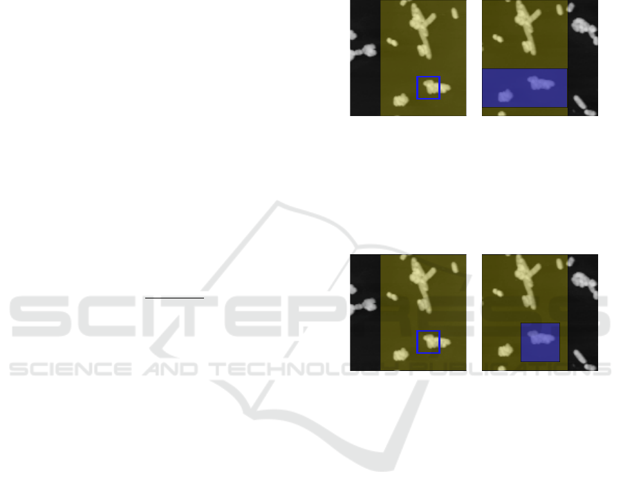
From assumption 1 the ROI can be limited to either

a horizontal or vertical slice (Figure 9) when only the

orientation of the two images are known (i.e. image 1

is to the left of image 2).

Image 1 Image 2

Figure 9: The highlighted area is the overlapping region,

the blue square is the template and the blue area is the ROI

in image 2.

If a rough translation is known as well (from a pre-

vious image pair) it is possible to estimate where the

template match is likely to be found on image 2 due

to assumption 2 (Figure 10).

Image 1 Image 2

Figure 10: The ROI in image 2 (blue area) is narrowed down

even further than in the previous ﬁgure.

The translation is therefore estimated as follows:

1. Limit the ROI on both image 1 and 2 to the over-

lapping region.

2. If a rough translation is known, jump to step 5.

3. Calculate the initial overlap from meta data from

the image ﬁles and adjust ROI accordingly on im-

age 1.

4. Use assumption 1 to limit the ROI on image 2.

Skip the next step.

5. Use assumption 2 to limit the ROI on image 2.

6. Extract a template T from image 1.

7. Find a match for T in image 2.

8. Calculate translation based on the position of T

and the found match.

2.2.4 Multiple Templates

Using a single template match to calculate the trans-

lation should be sufﬁcient in theory. However, it is

VISAPP 2016 - International Conference on Computer Vision Theory and Applications

116

possible that a match is not correct due to some of the

following reasons:

• Living Samples - If the sample is alive and mov-

ing around, it it possible that a template might not

be present in both images.

• Noise - Random noise in the images could mess

up the template matching and yield a false-

positive match.

• ROI Selection - The ROI selection might not

be spot on and the same template might not be

present in the ROIs for both images.

To avoid the impact of these issues, a voting-scheme

is utilized to decide which translation to accept.

Translation candidates are repeatedly calculated and

then allowed to cast a vote. This process stops when

a single translation candidate reaches a set number of

votes w and wins, or until no more templates can be

extracted from image 1. In the latter case, the candi-

date with the most votes wins.

Each vote cast is weighed:

weighted

= (m

rate

)

(10)

where v

weighted

is the weighted vote and m

rate

is the

similarity measure returned by the NCC in Equa-

tion 9. m

rate

is squared in order to punish translations

with a low match rate even further.

2.2.5 Stitching

The last step of the proposed solution is the actual

stitching of the images according to the found trans-

lations. The images are stitched together two images

at a time, ﬁrst horizontally into rows and then verti-

cally (Figure 11).

1 2 3

4 5 6

7 8 9

1 2 3

4 5 6

7 8 9

1 2 3

4 5 6

7 8 9

Figure 11: Stitching order.

The stitching order is similar to the order in which

the images are captured by the AFM, i.e. row-by-row.

This is an intentional choice, as it reduces the impact

of movement from living objects. The impact is re-

duced as the elapsed time between the capturing of

e.g. image 1 and 2 is less than the time between im-

age 1 and 4, thereby leaving less time for the objects

to move.

Two blending methods have been proposed:

mean

+ P

(11)

min

= min(P

) (12)

where P

is the respective pixel from the overlapping

part of image 1 and P

the pixel from image 2.

mean

is used in cases where the trails of move-

ment (ghosting artifacts) should be visible whereas

min

is used where these trails are unwanted. A down-

side of the P

min

method is that parts of the objects can

disappear as the minimum value of the two pixels is

used. An example of the two blending methods can be

seen in Figure 12, where a slightly wrong translation

is used to highlight how the methods behave.

mean

(a) Mean blending.

min

(b) Min blending.

Figure 12: The two blending methods used on the same

overlapping region.

3 RESULTS

A demonstration of how the proposed solution works

is illustrated in the bacteria images in Figure 13. The

result can be seen in Figure 15 and Figure 16 where

the mean and min blending methods have been used,

respectively.

The difference between the two blending methods

is not as clear as in the example in Figure 12 although

some lines, where the images are stitched, can be seen

when the mean blending method is used. These lines

occur as a result of the missing or moving objects as

explained earlier.

The solution is also tested on a dataset exhibit-

ing a high percentage of objects (Figure 14), which

is known to cause trouble for the leveling algorithm.

The purpose is to test the translation estimation and

stitching capabilities when the intensity is not consis-

tent due to the shortcomings of the leveling.

The result of the leveling and stitching process can

be seen in Figure 17. It is clear that the leveling al-

gorithm struggles, which is evident due to the many

artifacts. Most notable are the sharp seams caused by

different intensities and sudden ﬂuctuations in inten-

sity between lines. However, the translation estima-

tion and stitching does appear successful, as the ob-

jects agree with the objects found in the original 3x3

image grid.

A runtime test of the entire system is performed

on a laptop with a P8600 @ 2.4GHz using grids of

Stitching Grid-wise Atomic Force Microscope Images

117

3x3 images. Four different image grids were used,

one with a resolution of 512x512 pixels and three of

256x256 pixels. The high resolution grid took 43 sec-

onds to process, while the three lower resolution grids

took 13 seconds on average.

Figure 13: Topography images of bacteria - 3x3 grid.

Figure 14: Topography images of CHO cells - 3x3 grid.

4 DISCUSSION

The leveling algorithm starts to fail when the objects

occupy a percentage above 90% of each line (Fig-

ure 18). This high percentage increases the risk of

ﬁnding an inferior solution in the initial step where

RANSAC is used.

Figure 15: Stitched image of bacteria using the mean blend-

ing method.

Figure 16: Stitched image of bacteria using the min blend-

ing method.

Figure 17: Stitched image of CHO cells using the min

blending method.

A possible solution could be to apply RANSAC,

with fewer iterations, at several random lines in the

image, in order to ﬁnd a line with a decent amount of

background. Further tests on diverse datasets could

be used to identify the actual limit of the leveling al-

gorithm. Another issue is the impact of the points,

which are mistakenly classiﬁed as inliers (Figure 19).

In images with a relatively low object percentage this

is not an issue, as the false inliers will be outweighed

by the true inliers when ﬁtting a polynomial.

Reducing the threshold used when identifying in-

VISAPP 2016 - International Conference on Computer Vision Theory and Applications

118

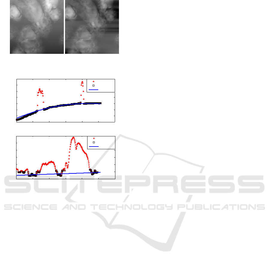
(a) Original image. (b) Leveled image.

Figure 18: Image with a high object percentage.

0 50 100 150 200 250 300

120

140

160

180

200

220

240

260

line

inliers

last poly

(a) Image 1 - easy to level.

0 50 100 150 200 250 300

120

140

160

180

200

220

240

line

inliers

last poly

(b) Image 2 - difﬁcult to level.

Figure 19: Example of inlier detection.

liers could be a possible solution to this problem, but

it has not been tested. Even if the leveling fails to

some degree, the NCC allows for intensity irregular-

ities between the images and is able to ﬁnd the right

translation. An improvement on the template recog-

nition could be to check the uniqueness of extracted

templates before attempting to match them.

The choice of the NCC and the region-of-interest

selection is based on the assumption that the im-

ages are only related through translation. This sim-

ple model seems to be a good choice as the images

appear to be correctly stitched when disregarding ar-

tifacts not caused by the stitching, like failed leveling

or disappearing objects.

The mean blending method is able to show how ob-

jects have moved between the images and the min

method can be used in cases where the overview is

more important than the detail. However, a blending

method that maintains the original shape of the ob-

jects, without ghosting artifacts, such as de-ghosting

(M. Uyttendaele and Szeliski, 2001) could improve

the output in certain scenarios.

5 CONCLUSION

The proposed solution is able to level and stitch grid-

wise captured AFM images with a few limitations as

discussed above. It takes between 12-43 seconds for

the system to stitch a grid of 3x3 images depending

on the size of the images.

The two blending methods work as intended al-

though there are disadvantages to both of them. The

decision of which method is the best in a speciﬁc sit-

uation depends on the user of the system.

REFERENCES

Briechle, K. and Hanebeck, U. D. (2001). Template match-

ing using fast normalized cross correlation. Optical

Pattern Recognition XII, 4387:95–102.

Brown, M. and Lowe, D. G. (2007). Automatic panoramic

image stitching using invariant features. International

Journal of Computer Vision.

Eaton, P. and West, P. (2010). Atomic Force Microscopy.

Oxford University Press.

Fischler, M. A. and Bolles, R. C. (1980). Random sample

consensus: A paradigm for model ﬁtting with appli-

cations to image analysis and automated cartography.

http://www.dtic.mil/dtic/tr/fulltext/u2/a460585.pdf.

Johnson, W. T. (2011). Imaging cells with the agilent

6000ilm afm.

Last, J. A. et al. (2010). The applications of atomic force

microscopy to vision science. Invest Ophthalmol Vis

Sci, 51:6083–6094.

Lowe, D. G. (1999). Object recognition from local scale-

invariant features. The Proceedings of the Seventh

IEEE International Conference on Computer Vision.

Lundtoft, D. H. (2014). Internship report from keysight

technologies. Technical report, Aalborg University.

M. Uyttendaele, A. E. and Szeliski, R. (2001). Eliminat-

ing ghosting and exposure artifacts in image mosaics.

Computer Vision and Pattern Recognition, pages 509–

516.

Pan, X. (2014). Processing and feature analysis of atomic

force microscopy images. Master’s thesis, Missouri

University of Science and Technology.

Tsaftaris, S. A. et al. (2008). Automated line ﬂattening

of atomic force microscopy images. Master’s thesis,

Northwestern University.

Stitching Grid-wise Atomic Force Microscope Images

119