Generating Straight Outlines of 2D Point Sets and Holes

using Dominant Directions or Orthogonal Projections

Melanie Pohl and Dirk Feldmann

Fraunhofer IOSB, Department Scene Analysis, Ettlingen, Germany

Keywords:

Point Set, Outline, Boundary, Hull, Concave, Building, Footprint, Dominant Direction, Preference Angles.

Abstract:

Representing the shape of ﬁnite point sets in 2D by simple polygons becomes a challenge if the resulting

outline needs to be non-convex and straight with only few, distinct edges and angles. Such outlines are usually

sought in order to border point sets that originate from man-made objects, e.g., for the purpose of building

reconstruction from LIDAR data. Algorithms for computing hulls of point sets obtained from such structures

usually yield polygons having too many edges and angles and may thus not capture the actual shape very well.

Furthermore, many existing approaches cannot handle empty domains within the boundaries of a point set

(holes).

In this paper, we present methods that create straight, non-convex outlines of ﬁnite 2D point sets and of

possibly contained holes. The resulting polygons feature fewer vertices and angles than hulls and can thus

faithfully represent objects of angular shapes.

1 INTRODUCTION

The problem of ﬁnding simple, planar polygons that

outline a ﬁnite point set in 2D Euclidean space arises

in many practical applications. In order to automati-

cally create polygonal 3D models (meshes) of build-

ings or even entire cities, for instance, it is com-

mon practice to employ point data acquired by LI-

DAR devices or from aerial photographs by means

of photogrammetric methods. These points are usu-

ally based in a plane section in 2D Euclidean space.

The task of creating meshes from such ﬁnite point

sets comprises the detection of their outlines (also

called footprints) (Vosselman, 1999). The most no-

table solutions to this kind of problem are probably

convex hulls. In the case of constructing 3D models

of buildings, convex hulls may be inappropriate, be-

cause the outlines of many buildings or building com-

plexes are not convex. A better approach would be

the usage of methods for ﬁnding non-convex (con-

cave) hulls. But since man-made objects like build-

ings tend to have lots of long, straight edges, which

furthermore enclose few angles of discrete measures

(e.g., ±

), true hulls rarely reﬂect the desired out-

lines very well as shown in Figure 1: The outline

of the building obtained by the Concave Hull Algo-

rihtm (Moreira and Santos, 2007) is clearly prefer-

able over the convex hull, but it has too many ver-

tices and is not as straight as the underlying build-

ings’ exterior boundaries really are. For the task of

building reconstruction, having nicely straight out-

lines with only few vertices is desirable, because it

simpliﬁes the process of 3D model generation and

the results are more realistic. Straightening outlines

obtained from concave hulls using methods like the

popular Ramer-Douglas-Peucker Algorithm (Ramer,

1972; Douglas and Peucker, 1973) is not a general

solution due to unintentional removal of certain cor-

ners as shown in Figure 1(b). Please note that we do

not deal with buildings having strongly curved bound-

aries, even though these can be found in many archi-

tectural landmarks.

Furthermore, input data obtained by measure-

ments are always noisy and the distribution of points

is likely to be non-uniform. Since hulls must include

every point of the set they enclose, unwanted outliers

will further diminish the desired quality of the result-

ing outlines.

The boundaries of ﬁnite point sets located in

a plane section in 2D Euclidean space may also

feature larger domains where no points are present

at all (called holes). In the process of building

reconstruction from LIDAR data, for instance, such

empty domains frequently result from buildings

or building complexes having inner courtyards or

atria. In order to give faithful representations of

Pohl, M. and Feldmann, D.

Generating Straight Outlines of 2D Point Sets and Holes using Dominant Directions or Orthogonal Projections.

DOI: 10.5220/0005720300570069

In Proceedings of the 11th Joint Conference on Computer Vision, Imaging and Computer Graphics Theory and Applications (VISIGRAPP 2016) - Volume 1: GRAPP, pages 59-71

ISBN: 978-989-758-175-5

(a) convex hull. (b) concave hull (k = 100). (c) our method (orthogonal

projection).

Figure 1: Using the convex hull or the Concave Hull Algorithm to generate outlines of 2D point sets obtained from man-made

structures, like buildings, leads to shapes that do not necessarily reﬂect the actual object very well. Straightening the resulting

outlines using Ramer-Douglas-Peucker Algorithm (blue line in (b)) only little improves the result. Our method based on

orthogonal projection creates outlines that represent such objects more accurately. In Figure 1(b), k denotes the number of

neighbors considered (see Section 2.1).

the underlying objects, these holes also need to be

bounded by simple polygons.

We present two methods for ﬁnding simple out-

line polygons of 2D point sets which feature fewer

vertices and angles than hulls in order to faithfully

represent shapes of structures that are typically man-

made or originate from technical processes. These

structures may contain holes and are characterized by

straight edges and may be non-convex. Frequently,

they are moreover (near-)rectangular and have only

few angles and corners. Our methods are based on

the Concave Hull algorithm presented in (Moreira and

Santos, 2007). Although our application aims at gen-

erating outlines for the task of building reconstruc-

tion, and we therefore demonstrate and evaluate our

method in the context of that application, the proceed-

ings presented in this work are general and versatile.

2 RELATED WORK

Finding outlines of 2D point sets representing struc-

tures that have straight edges and enclose only few an-

gles in order to obtain “good” representations of the

underlying objects is an inherently ambiguous prob-

lem and strongly depends on the application. As

pointed out in (Galton and Duckham, 2006), there is

no single correct outline or footprint of a set of points.

Computing outlines by means of convex hulls, for in-

stance, is probably reasonable if the underlying ob-

jects are (almost) convex themselves. Convex hulls

are well-studied and many algorithms are known for

its computation (de Berg et al., 2008), but in case of

non-convex objects, convex hulls naturally yield un-

satisfactory outlines. Therefore, we do not further en-

ter on methods for their generation.

α-shapes (Edelsbrunner et al., 1983) are a gen-

eralization of convex hulls and allow for computing

non-convex (concave) outlines of 2D point sets. The

α-shape of a ﬁnite point set S ⊂ R

is the boundary

of the α-hull of S. The latter can be obtained by com-

puting the Delaunay triangulation of S and removing

those k-simplexes, 0 ≤ k ≤ 2, whose open circum-

scribed circles have radii ≥

or that contain any other

p ∈ S. Using α = 0, the α-shape of S is deﬁned to be

its convex hull.

Another approach based on Delaunay triangula-

tion are characteristic shapes (χ-shapes) as presented

in (Duckham et al., 2008). The algorithm repeat-

edly removes the longest exterior edge whose length

is greater than some value L from the initial Delaunay

triangulation of S , provided that the remaining exte-

rior edges form a simple polygon. It is also possible to

parametrize χ-shapes by a normalized length parame-

ter λ =

l−l

min

max

−l

min

, where l denotes the length of an edge

and l

min

and l

max

are the minimal and maximal edge

length from the Delaunay triangulation, respectively.

The resulting outlines produced by α- and

χ-shapes depend on the choice of the respective

parameters α and l (or λ). Their choice involves

a-priori knowledge about the shape of the underlying

point set, or appropriate values must be found using

heuristics or by trial and error.

The Concave Hull Algorithm in (Moreira and

Santos, 2007) is based on the idea of Jarvis’ March

aka. Gift Wrapping Algorithm (Jarvis, 1973) for com-

puting convex hulls: Instead of considering all ele-

ments from the set of remaining points S , the Con-

cave Hull Algorithm only considers the 3 ≤ k ≤

nearest neighbors of the point that has been added

to the hull last. Using greater values for k results in

larger neighborhoods being considered, and the con-

GRAPP 2016 - International Conference on Computer Graphics Theory and Applications

cave hull becomes “more convex” as k increases. If

k =

, the algorithm computes the convex hull, be-

cause the set of points considered becomes the same

as with Jarvis’ March. Since our method is based on

the Concave Hull algorithm, it is brieﬂy summarized

in Section 2.1.

The strength of Concave Hull is its simplicity

and that there is no need to compute any (Delaunay)

triangulation of which most information about con-

nectivity is not needed at all.

In (Asaeedi et al., 2013), the Alpha-Concave Hull

is presented, which is a simple polygon whose interior

angles are < π+α. If the parameter α = π, the Alpha-

Concave Hull is the minimal polygon of S ; in case of

α = 0, it is the convex hull.

In the ﬁeld of photogrammetry, methods for gen-

erating rectangular outlines of buildings based on line

ﬁtting of contour points, like the one presented in

(Vosselman, 1999), seem to be popular. The draw-

back of these methods is their limitation to the cre-

ation of only rectangular outlines. But even in the

application of detecting building outlines, there are

often boundaries that are not rectangular, at least in

some corners, like in cities that grew over centuries or

that were not planed from scratch.

There are also approaches based on statistical

estimates of the most appropriate outline for a given

set of points (Wang et al., 2006).

Furthermore, among the methods presented so far,

only α-shapes can create outlines of holes in 2D

(see Section 1), but the resulting outlines are overly

jagged. Representing holes, however, is essential

to obtain faithful representations of atria or build-

ing complexes enclosing inner courtyards. The so-

lutions presented in (Bendels et al., 2006), (Wang and

Oliveira, 2007) and (Wu and Chen, 2014) address the

detection (and also ﬁlling) of holes in point clouds

that represent surfaces in 3D, so that these methods

are difﬁcult to apply to our problem.

2.1 Concave Hull Algorithm

To generate outlines, also called boundaries in the re-

mainder of this work, we adopt the Concave Hull Al-

gorithm in (Moreira and Santos, 2007) which is sum-

marized below, because it is the foundation of our ap-

proach. For a more detailed description, we refer to

the original article.

Let S be a ﬁnite set of points in 2D Euclidean

space where p

6= p

∀p

, p

∈ S ∧ i 6= j. Let further-

more p

∈ S be the point having minimal y-coordinate

and C

= (v

,. . ., v

) the list of vertices of the out-

line computed so far.

Given k ∈ N, 3 ≤ k <

, start with n = 0, n ∈ N,

−1

= S, C

= (v

= p

), p = p

and e = −x, where

−x denotes the negative x-axis. Remove p from the

current set of points to obtain S

= S

n−1

\p and com-

pute the set K

(p) ⊂ S

of p’s k nearest neighbors.

The points q

∈ K

(p), 0 ≤ i < k are sorted accord-

ing to the clockwise angle ϕ

enclosed between the

directed edge e

= (q

− p) and edge e such that j = 0

be the index of the point p

= q

where ϕ

is largest,

j = 1 the one where ϕ

is second largest, etc.

Now let e

= (p

− p) denote the directed edge

from the last vertex of the outline polygon to the

point p

∈ K

(p), j = 0,1, . .. k. Starting at j = 0,

check if e

does not intersect any of the existing edges

n−2

n−3

n−4

,. . ., v

of the polygon. If e

in-

tersects an existing edge of the hull, retry using e

j+1

if j < k. In case no e

remains, the outline computed

so far is discarded, k is increased and the algorithm is

restarted using n = 0 again. Otherwise, if no intersec-

tion of e

with an existing edge is found, set p

= p

to be the best match in K

(p), add p

to the list of

vertices, i.e., C

n+1

= C

∪ p

, and set e ← (v

− p

)

as the backwards directed edge formed by the last two

vertices of the hull. The process is then restarted set-

ting n ← n + 1 and p ← p

until p = p

again or all

points in S haven been processed. In order to ensure

that p = p

a second time and that the algorithm ter-

minates, p

must be added to S

again after the third

iteration. When p = p

the second time, it is neces-

sary to check if all remaining points in S

are actually

inside the resulting polygon C

so that it is actually a

hull in the proper sense. Otherwise, the outline is also

discarded, k is increased and the algorithm is restarted

using n = 0.

3 COMPUTING OUTER

BOUNDARIES

In this section we present two different approaches for

computing simple polygons that outline a given ﬁnite

point set S ⊂ R

. The outline’s edges only enclose

angles of a few, distinct values, and we call them an-

gular outlines in the following.

The ﬁrst method relies on the concave hull and de-

termination of dominant edge directions. Our second

method modiﬁes the Concave Hull Algorithm to di-

rectly compute an angular outline.

The advantage of the ﬁrst method, presented in

Section 3.1, is that the hull can be straightened by

two predeﬁned main angles. This idea follows the ap-

proach, that buildings are mostly oriented along two

Generating Straight Outlines of 2D Point Sets and Holes using Dominant Directions or Orthogonal Projections

directions to guarantee parallel walls. Furthermore, if

we also take the idea of perpendicularity into account,

we can force the straightened edges to form right an-

gles. Therefore, data that are very noisy or contain

holes can be bordered along the main directions or

perpendicular to it.

The second approach in Section 3.2 is preferable

if the underlying structure is not well approximated

by strictly rectangular outlines or if the edges of the

shape enclose more than two distinct angles. How-

ever, for this method to work, the initial orientation

of the underlying shape within a Cartesian coordinate

system must be provided.

3.1 Angular Outlines from Dominant

Directions

Let C

be the list of vertices of a concave hull of S and

E = (e

,..., e

) the list of edges with e

= v

i+1

, i =

0,1, . .. , (m − 1) and e

= v

. Since we do not

consider the orientation of an edge, each difference

vector e

is set to e

← sgn (e

i,y

) · e

. For each edge

, we compute the angle α

∈ [0,π] that is enclosed

with the positive x−axis. If α

= π, we set α

← 0.

The length of an edge e

is denoted by l

. We an-

alyze the directions and lengths of each edge of the

concave hull polygon and compute a length-weighted

angle histogram H(α

). Angle α

is assigned to the

respective bin of width w according to

−

+ (2n − 1) ·

≤ α

< (2n − 1) ·

n ∈ {1,2, ..., m}.

The value of the n-th bin is computed as

∑

From this histogram, we compute the two domi-

nant angles β and γ of the concave hull using one of

the following two options:

1. Approximate the histogram H(α

) by a bimodal

distribution. Then β and γ correspond to the an-

gles of the two maximums of the approximation.

2. β corresponds to the angle of the maximum value

in H and γ is offset by ±

β = argmax

0≤α

<π

(H (α

)), γ =

(

β +

, β <

β −

, β ≥

The advantage of option 1 (“peaks” option) is that the

edges of the boundary obtained from straightening of

the concave hull can enclose an arbitrary but ﬁxed an-

gle that equals

β − γ

. Option 2 (“90

◦

” option) en-

sures that these edges always enclose right angles.

From β and γ we compute the corresponding dom-

inant directions



cos(ϕ)

sin(ϕ)



, ϕ ∈

{

β,γ

}

and assign labels ρ

to all edges of the concave hull

according to the dominant angle they belong to:

= argmin

{](e

)}, ϕ ∈ {β, γ}.

To simplify the straightening procedure it is advis-

able to shift the start point in the sequence of vertices

of the concave hull and the entries of the label vec-

tor to ensure a tuple of successive vertices having the

same label is not split by the start or end vertex. Af-

terwards, we collect every tuple of successive vertices

= (t

,...) from the concave hull that belong to

the same label ρ

and compute the line ` through the

center of gravity along the corresponding main direc-

tion d

` :~x =

∑

∈T

+ µ d

To limit these lines, we have to distinguish two

cases: If the foregoing (or subsequent) tuple belongs

to none of the dominant angles/directions we project

the ﬁrst (or accordingly the last vertex) onto that line.

If the foregoing (or subsequent) tuple belongs to the

other dominant angle/direction, the end points are

speciﬁed by the intersection point of the line corre-

sponding to the foregoing (or subsequent) tuple and

the current tuple’s line.

3.2 Angular Outlines from Orthogonal

Projection

Our second approach to computing angular bound-

aries modiﬁes the Concave Hull Algorithm in Sec-

tion 2.1 by projecting the edges of the hull onto or-

thogonal line segments and adjusting them. First, we

explain the process of projection onto orthogonal line

segments. This yields a strictly rectangular outline,

which is only a “good” representation if the underly-

ing shape is (almost) rectangular, too. The proceeding

is then extended by three modiﬁcations that improve

the shape of the outline in situations where strictly

rectangular outlines may be perceived as unsatisfac-

tory representations.

3.2.1 Orthogonal Projection

In this section, we use the same symbols from the

description of the Concave Hull Algorithm in Sec-

tion 2.1. In addition, let δ

= i ·

,i = 0,1, . .. , 4.

GRAPP 2016 - International Conference on Computer Graphics Theory and Applications

When the Concave Hull has determined a candidate

among the sorted k nearest neighbors K

(p) of the

current point p ∈ S

that satisﬁes the requirements for

being a new vertex of the outline polygon, we modify

the algorithm to additionally compute

= argmin





− ϕ





where ϕ

is the angle associated with p

such that δ

the angle that deviates least from ϕ

. If δ

happens to

be 0 or 2π, we discard p

and proceed with the next

candidate in K

(p), if there is any left. Otherwise, p

is discarded from the set of remaining points, just like

with the Concave Hull.

Using δ

, we compute the corresponding direction

d and an orthogonal vector u pointing to the “right-

hand side” of the ray R from p in direction d, away

from where the majority of points of S is located:

d =



cos(θ)

sin(θ)



, u =



sin(θ)

−cos (θ)



where θ = θ

+ (π − δ

) and θ

is the angle enclosed

by the last edge e of the outline computed so far and

the x-axis. Please notice that we have to use π − δ

instead of δ

to compute θ, because we chose clock-

wise angles in [0,2π] with the Concave Hull Algo-

rithm. The outer boundary is thus oriented counter-

clockwise. The vector e

= (p

− p), which corre-

sponds to edge p

p, is then projected onto d and u

to obtain the lengths l

= d · e

and l

= u · e

, re-

spectively. Next, the new vertex q to be added to the

current outline C

= (v

,. . ., v

) is computed as

q = p +

· d + w

where

w =

(

max(l

,0) · u, δ

= π

· u, otherwise

(1)

Thus, if an edge is continued (i.e., δ

= π), w is either

zero or points towards the right-hand side. Otherwise,

if the new edge introduces a turn, it may also point to

the left-hand side of R. The outline polygon is then

updated by considering the following two cases:

1. If C

contains ≥ 2 vertices and the edge is about

to be continued, we replace the last vertex by q

and add w to the second last vertex:

← q, v

n−1

← (v

n−1

+ w) (2)

2. Otherwise, if δ

or δ

3π

and the outline is

about to make a left or right turn, respectively, or

if it contains only one vertex so far, we append q

to C

and add w to v

n+1

= q, v

← (v

+ w) (3)

In the next iteration n + 1, we proceed with q instead

of p

, after having removed p

from the point set

n+1

. As with the Concave Hull algorithm, we check

for self-intersections of the resulting polygon. In pos-

itive cases, we also discard the polygon and start the

algorithm from the beginning using k + 1. Likewise,

we terminate if p

= p

again, but since C

is obvi-

ously not a hull, it does not necessarily include all

points in S . Therefore, we omit the ﬁnal check of

whether all points in S are located strictly inside C

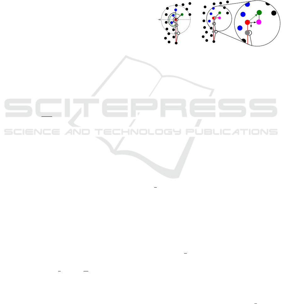
Figure 2 illustrates the proceeding described above.

–

–π

–

–π

Figure 2: Creating angular outline by means of orthogonal

projection is based on the Concave Hull Algorithm, but in-

stead of adding p

to the list vertices, its projection q onto

d is added.

Due to the choice of w in Equation 1, we ensure

that edges are dragged only to the “outside” of the

shape and that more points (including p

) are located

“inside” the resulting outline, if an edge is continued.

In case of left or right turns, an edge may also be-

come dragged towards the “inside” (l

< 0) in order

to enclose the point set S more tightly. However, this

may cause some points of S to be found again among

the k nearest neighbors K

n+1

(p) in the next iteration.

Depending on the choice of k, this can lead to self-

intersections and the rejection of the current k. The

results of this proceeding are satisfactory in case of

shapes that are (almost) rectangular everywhere. In

cases where a shape’s corners deviate too much from

, e.g., in case of point sets derived from ancient or

architecturally unusual buildings, the outlines are less

appealing (see Figure 3).

3.2.2 Improvements for Non-Rectangular

Shapes

To make the outline match non-regular shapes more

accurately, e.g., if one or more corners deviate too

much from ±

, we introduce some modiﬁcations to

the proceeding described in Section 3.2.1. First, we

can simply omit the addition of w to the predecessor

of the last vertex in Equation 2 when an edge is con-

tinued. As a result, the continued edge is not neces-

sarily perpendicular to the previous one anymore, but

the outline captures a shape more accurately at cor-

ners where two edges join at angles ϕ >

. Corners

Generating Straight Outlines of 2D Point Sets and Holes using Dominant Directions or Orthogonal Projections

(a) (b)

Figure 3: Pure orthogonal projection and dragging contin-

ued edges only to the outside yields appealing results if the

underlying shape is almost rectangular itself (a), but causes

the appearance of unwanted steps if corners are present that

are not rectangular (b).

where ϕ <

remain approximated by steps, because

the line segment of a continued edge is only allowed

to being dragged outside due to Equation 1. Thus, we

modify Equation 1 to obtain Equation 4:

w =

(

max(l

,0) · u, if δ

= π ∧ outside = true

· u, otherwise.

(4)

The predicate outside is set to false if δ

or δ

3π

. It is set to true if δ

= π and if l

> 0 for any point

along the continued edge. In this way, a continued

edge may also become dragged towards the inside and

enclose S more tightly, as long as there is no need to

drag the edge outside again, i.e., l

< 0 over the whole

distance the edge is continued.

Dragging the last vertex of a continued edge to-

wards the inside can cause more points of K

(p) to

lie on the right-hand side of the edge, because p

not necessarily the ﬁrst point in the descending or-

der of enclosed, clockwise angles. Those points may

be found in the next iteration in K

n+1

(p) again, and

they may introduce unwanted turns and corners in the

outline, or disturb the algorithm by self-intersections.

Therefore, we not only remove p

from S

to obtain

n+1

, but also every other point p

∈ K

(p) whose

associated edge (p

− p) encloses a clockwise angle

with the outline’s last edge e = (p − v

n−1

) that is

larger than the one enclosed between e and (q − p).

A further adjustment that affects concavities of a

shape is the enforcement of creating steps in the out-

line by modifying Equation 2 to obtain Equation 5:

← q

n−1

←

(

n−1

+ w, second last trun was right

n−1

, otherwise.

(5)

In other words, we add w to the second last vertex of

a continued edge, if the second last turn of the out-

line we encountered was a right turn, and the edge

is thus part of a concavity. In such concave regions,

the algorithm then behaves like the version in Sec-

tion 3.2.1, and problems as shown in Figure 4 are pre-

vented. The beneﬁt of this modiﬁcation, however, de-

pends on the application and the underlying point set,

and to some degree on the user’s judgment or personal

preferences.

Figure 4: Due to dragging only the last vertex of outlines,

edges may be moved into concavities and can unintention-

ally cut off too many points.

3.2.3 The Choice of Initial Direction

In the proceeding described in Section 3.2.1, the ini-

tial direction given by θ

is yet unspeciﬁed, but it in-

ﬂuences the resulting outline as shown in Figure 5.

Using θ

= 0 is only reasonable if the lowest edge of

shape is (near) parallel to the x-axis. But since the ori-

entation of the shape we are trying to approximate by

angular outlines may be unknown in advance, we ei-

ther have to let the user specify θ

or obtain it from

analysis of the point set’s orientation by statistical

means, e.g., via principal component analysis (PCA)

or the methods employed in Section 3.1.

Figure 5: The shape represented by the point is actuall tilted

by ≈ 25

◦

against the x-axis. Not accounting for this initial

orientation yields unpleasant results.

Starting at point p

having lowest y-coordinate, we

might also run our algorithm using θ

= 0. The ﬁrst

time we encounter δ

6= π, we can set θ to the angle

enclosed between the ﬁrst edge and the x-axis. In this

way, θ

not only depends on p

, but also on the choice

of the size of the neighborhood k, which can be un-

satisfactory as outliers in the neighborhood of p

may

GRAPP 2016 - International Conference on Computer Graphics Theory and Applications

yield an inappropriate outline. However, if the point

set is sufﬁciently clean and dense in the area of the

outline’s ﬁrst edge, this method works quite well. It

can also be used to give the user a hint of the initial

orientation of the shape.

3.3 Obtaining Simple Polygons

Due to the straightening process of the concave hull

(Section 3.1) or the dragging of edges (Section 3.2.1),

the outlines created by our methods may be self-

intersecting. To obtain simple polygons, these self-

intersections need to be detected, and the line seg-

ments between the points of intersection are cut off.

4 OUTLINES OF HOLES

The outlines of point sets in plane sections in 2D Eu-

clidean space may comprise larger areas where no

points are present. In the application of building

reconstruction from LIDAR data, for instance, this

happens if building complexes contain atria or inner

courtyards, because the data may only yield informa-

tion about distinctly elevated structures, like roofs.

We call such empty areas holes within the point set

and deﬁne them more formally as in Deﬁnition 1.

Deﬁnition 1. Let S ⊂ R

be a ﬁnite point set and

Ω(S ) ⊂ R

be the domain inside a simple polygon

that tightly encloses all elements of S (e.g., one of

its hulls or the minimal axis-aligned bounding box).

We call a connected region E ⊂ Ω(S) of ﬁnite area

a hole (in or of S ) of size r, if E is large enough to

fully overlap a circle of radius r > 0 at some location

c such that ∀p ∈ S :

p − c

≥ r.

r is called the size of hole E.

Our deﬁnition of hole depends on the choice of

polygon to border Ω(S): it is possible to choose dif-

ferent boundaries for S that have different numbers of

holes, or holes of different sizes. In this work, how-

ever, we are only interested in holes that do not border

on the enclosing polygons of point sets.

In order to obtain faithful outlines of the objects

represented by 2D points, we extend our methods by

creating inner boundaries. Since we are only inter-

ested in holes that are “large enough”, we choose a

minimum hole diameter d

min

that shall be detected.

The choice of d

min

depends on the application and the

average sampling density of the point set. In the ap-

plication of building reconstruction, for instance, d

min

might be related to the sizes of humans or vehicles,

if the holes originate from courtyards, because such

structures usually serve a purpose and thus need to be

accessible.

In contrast to outer boundaries, inner boundaries

shall be oriented clockwise. This is mainly due to

technical aspects and conventions, for it allows us to

easily determine whether a point is located inside or

outside the inner or outer boundary. Besides, we need

to take into account that there might be more than one

hole in a given point set.

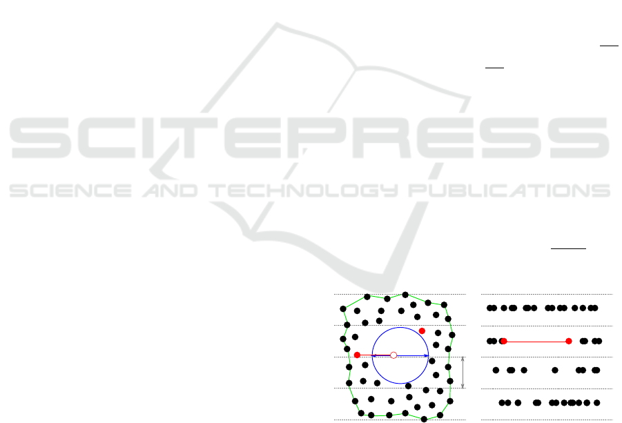
4.1 Detecting Holes

The basic idea of detecting holes is to ﬁnd points on

their border and to create their outlines by applying

modiﬁed versions of the methods presented in Sec-

tion 3. In order to ﬁnd points on the border of holes,

we employ the following heuristic (see also Figure 6):

1. Let h be the extent of point set S along the y-axis;

choose a minimum hole diameter d

min

. Let fur-

thermore P be a simple, closed outline polygon of

S, e.g., a (concave) hull or any other outline ob-

tained by our methods.

2. Split S along y-axis into m strips of width w =

min

in such a way that m =

min

∈ N.

3. Obtain disjoint point sets Y

for each of the 0 <

j ≤ m strips where ∀a, b ∈ [0, m − 1], a 6= b, Y

∩

a+1

0 ∧

m−1

j=0

= S.

4. For each set Y

, sort the points in Y

in ascending

order of x-coordinates.

5. For each two neighboring points p

, p

i+1

in Y

compute the distance d =

i+1,x

− p

i,x

6. If d ≥ 2 · w and m = (p

i,x

+ w, p

i,y

) is located in-

side P, add the directed line segment p

i+1

to the

list of candidates Q.

min

Figure 6: To ﬁnd locations on the border of a hole from

where to start the generation of inner boundaries, the point

set is cut into strips perpendicular to the y-axis (left). Neigh-

boring points whose projections onto the x-axis have dis-

tances ≥ d

min

are candidates (red), if m (red circle) is inside

the point set’s boundary (green).

This approach will ﬁnd the points on the borders

of all holes at once, but we cannot tell the hole a can-

didate belongs to. To solve this problem, we compute

Generating Straight Outlines of 2D Point Sets and Holes using Dominant Directions or Orthogonal Projections

an outline of the hole for the left vertex of ﬁrst line

segment s

= a

in Q as described in Section 4.2

and remove it from Q. For each of the remaining line

segments s

= a

∈ Q, j > 0, we check if the mid-

point m

of s

is located inside any previously com-

puted outline of a hole, and discard s

if m

is in-

side. Furthermore, we check if any edge of a new hole

boundary intersects an edge of a previously computed

hole outline. If two outlines intersect, we can discard

one of them based on a reasonable criterion, e.g., the

size of its area or its number of vertices. Another op-

tion would be to merge the two outlines in order to

obtain a common outline, but we did not implement

this approach due to its complexity.

Alternatively, we may suspend the search for

further candidates after the ﬁrst one. After generating

the hole boundary, we can ﬁll the hole with phantom

data points based on a point density estimation. The

next candidate is then detected by restarting the

search procedure from the beginning.

With the approach described above, we cannot

yet guarantee that the resulting outline borders a hole

overlapping a circle of radius ≥ w and is therefore

consistent with Deﬁnition 1: Due to “cutting” the

point set perpendicular the y-axis into strips of width

w =

min

, the hole has at least a radius of half the size

. Cutting the point set into strips of width d

min

might cause holes around this size to be missed, be-

cause the strips are projected onto the x-axis and gaps

might be concealed from projections of points on the

top or bottom of the hole. This is a sampling problem

and the strip width w should thus be smaller than

min

in a practical implementation.

Verifying the size of the hole found by the heuris-

tic above turns out to be difﬁcult, since we would need

to ﬁnd the center of an empty circle with radius d

min

within the hole, but there are potentially inﬁnite many

locations. By placing a circle of radius d

min

at the

centroid of the hole’s outline polygon, for example,

the hole can be accepted if the circle is empty, but it

cannot be safely reject, if the circle is not empty. In

practical applications that do not rely on the exact size

of a hole, it may still be sufﬁcient to ﬁnd holes that are

known overlap circles with radii the range of

and w.

4.2 Bordering Holes

Creating the outlines of holes is done using slightly

modiﬁed version of the procedures described in Sec-

tion 3 and the Concave Hull algorithm in Section 2.1.

The modiﬁcations basically account for changing the

orientation of the resulting polygon to clockwise, and

the different starting location.

Our modiﬁcation to the Concave Hull algorithm

to obtain a clockwise oriented polygon for outlining

holes is as follows: Among all k neighbors K

of the

current point p = v

, we search for the point q

with

the smallest counter-clockwise angle ϕ

= ](ξ

, e

) where ξ

is the previous edge directed back-

wards, i.e., ξ

= v

n−1

instead of v

n−1

. Initially,

we use the positive x−axis for ξ

By choosing p

as the ﬁrst vertex a

of the line

segments s

∈ Q obtained by the heuristic given in

Section 4.1, we start at a point that is part of the left

border of the hole. The point may furthermore be lo-

cated on a sharp crease (like a v-shaped corner) such

that the smallest ϕ

may be associated with a point

at the opposite border of that crease. Thus, the out-

line generation might fail right away, if k was too

large. Replacing ξ

by an edge that is rotated counter-

clockwise by

to point inside the hole yields better

results, but if the neighborhood gets even larger, the

algorithm can still fail for the same reason.

Due to its position on the left border of the hole,

the point p

= a

may not necessarily be found in a k

nearest neighborhood a second time. Therefore, we

also have to extend the condition for terminating the

hole’s concave hull computation: For each new line

segment added to the hull, we additionally check if it

intersects the line segment s

= a

∈ Q . Starting

from point a

, the edges of the outline to be created

will enter the “upper” part of the hole. They can only

enter the “lower” part by crossing s

on the right

border at b

or close to it. Once a line segment enters

the “upper” part from the hole’s “lower” part again,

is crossed a second time, and we terminate the hull

computation, because the polygon has encircled the

hole.

Using our method to generate the outline of a hole

by means of dominant directions as presented in Sec-

tion 3.1, we ﬁrst create a clockwise oriented concave

hull as described above, and apply the same proceed-

ing to straighten the concave hull of a hole afterwards.

Our method described in Section 3.2 merely needs to

be adjusted in the same way as the Concave Hull Al-

gorithm in order to create outlines of holes.

5 RESULTS AND DISCUSSION

We demonstrate the usability of our methods by

means of four different data sets D

– D

: the point

sets already depicted in Figures 3(a) (D

), 1 (D

) and

3(b) (D

), originate from airborne laser scans. The

point set depicted in Figure 12(a) (D

) is a synthetic

data set featuring a star-shaped hole. Data sets D

–

GRAPP 2016 - International Conference on Computer Graphics Theory and Applications

represent non-convex building complexes, but D

is moreover near-rectangular in contrast to D

and D

For the purpose of generating ﬁgures, we reduced the

number of points depicted, but to create outlines, we

always employed the original, denser point sets.

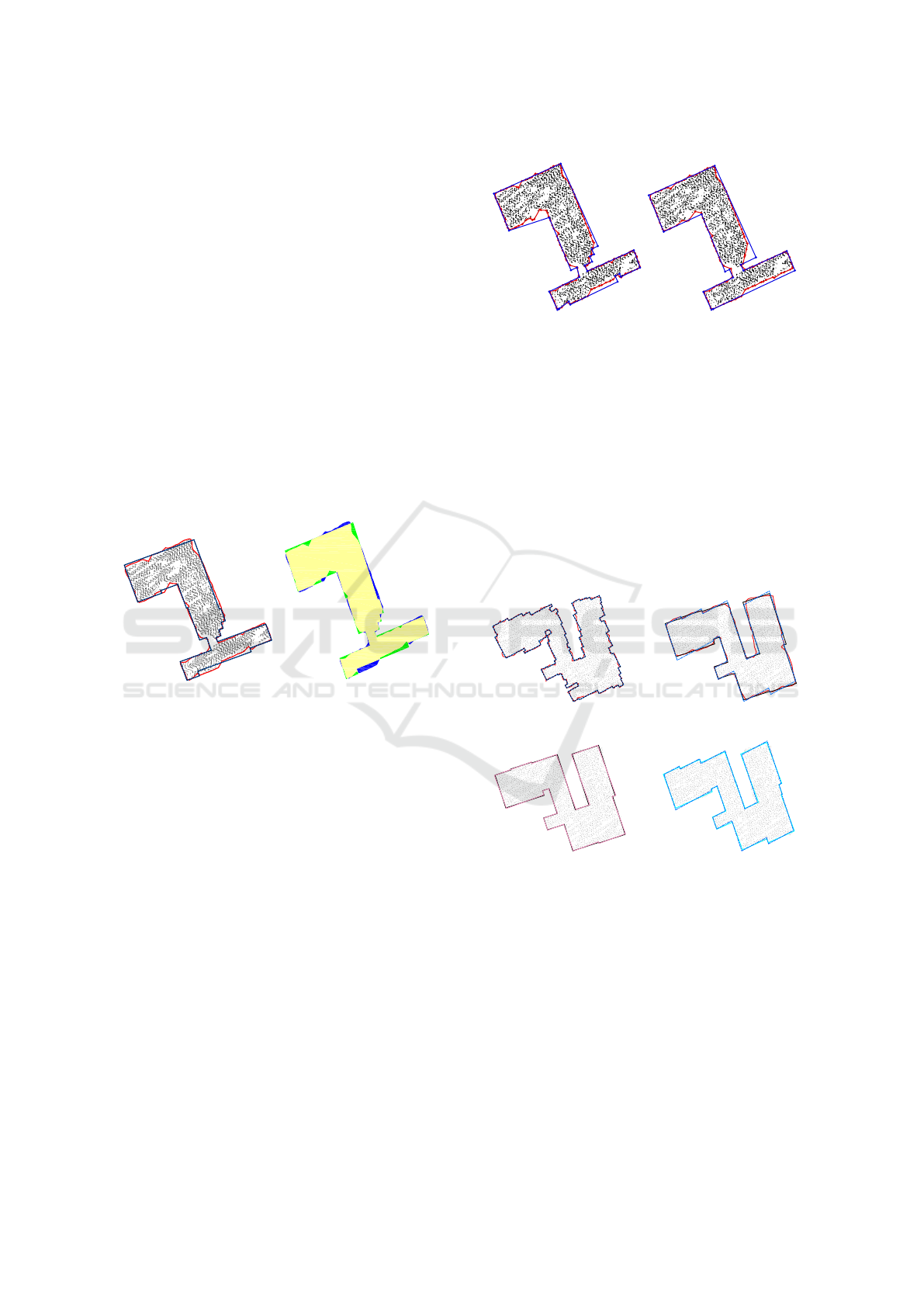
5.1 Results

The outline of D

generated by means of domi-

nant directions (see Section 3.1) is shown in Fig-

ure 7(a). With this data set, both options for determin-

ing the dominant directions (“peaks” and “90

◦

”) lead

to the same rectangular outline that is signiﬁcantly

“straighter” than the concave hull for k = 60, but

satisfactorily represents the underlying shape. The

straightening process causes changes in areas as high-

lighted in Figure 7(b). These changes are small but

help to approximate the building’s true outline and

compensate for noise and mistaken measurements.

(a) outline dominant direc-

tions

(b) differences of over-

lapped areas

Figure 7: The concave hulls (red) of D

using k = 60 com-

pared to outlines generated by means of our method using

dominant directions. Left: the two options “90

◦

angles”

(black dotted) and “peaks” (blue) lead to same outline with

substantially fewer vertices than the concave hull. Right:

areas overlapped by the concave hull (yellow + blue) and

the straightened outline (yellow + green).

Like with the original Concave Hull algorithm,

we can inﬂuence the shape of the resulting outlines

by altering k. Using larger k yields boundaries that

look “more convex” than the ones created using

smaller k. This is illustrated in Figure 8 by means

of outlines of D

obtained by using orthogonal

projection (Section 3.2).

Boundaries of D

using dominant directions are

given in Figure 9. With this data set, the ﬁrst main

direction is almost independent of k, but increasing

k also increases the uncertainty in the determination

of the second main direction. Since the later is also

inﬂuenced by the point distribution and data noise,

at larger k, the resulting outline looks a somewhat

(a) k = 60 (b) k = 100

Figure 8: Outlines of D

generated by using our method

based on orthogonal projection (blue) compared to the con-

cave hull (red) at different values of k.

skewed against the point set’s shape. In this case, the

outline created by using our “90

◦

” option encloses the

points more accurately. The remaining deviations re-

sult from the fact that the shape of D

is not truly rect-

angular. Figure 1(c) depicts an outline of this data set

generated by means of orthogonal projection. Since

the edges of that outline do not necessarily join or-

thogonally due to the dragging operations performed,

it captures the point set’s shape very well.

(a) k=20 (b) k=100

ing: 90

◦

; bin width

◦

(black) : 1

◦

(pink)

(d) k = 100, straight-

ening: main angles;

bin width 10

◦

(blue) :

◦

(cyan)

Figure 9: Straightened building outlines from the concave

hull (red) for k = 20 (a) and k = 100 (b) neighbors. Larger

k lead to smoother outlines but increase the uncertainty for

computing the main direction. Changing the bin sizes leads

to a tilt of the boundary.

is a real-world example of a point set acquired

from a non-rectangular, non-convex building that has

an atrium. Outlines of the outer and inner boundaries

created by means of our methods are shown in Fig-

ure 10. Figures 10(a) and 10(b) show the concave

hull and outlines of holes of minimum diameter d

min

Generating Straight Outlines of 2D Point Sets and Holes using Dominant Directions or Orthogonal Projections

of 100 units and 30 units, respectively. These bound-

aries were created by means of our dominant direc-

tions method, and the holes were found using our

heuristic in Section 4.1. Using a smaller hole size,

we are able to ﬁnd and outline the additional hole in

the upper right corner, whereas a larger hole size only

allows for handling the atrium. However, the inner

and outer boundaries produced by the straightening

procedure do not faithfully represent the shape of the

underlying building: The lower part of the polygon

is approximated quite well when the concave hull is

straightened by using the “90

◦

” option, whereas the

upper edge is matched unsatisfactorily. Using the

“peaks” option, we have the opposite situation, and

the upper edge is matched quite well, although the

ﬁrst main direction is equal with both options. Since

our approach based on dominant directions only al-

lows to straighten along two dominant directions, it

cannot match both edges at once.

(a) d

min

= 100 (b) d

min

= 30

Figure 10: Concave hull (red) and straightened outlines ob-

tained from dominant directions and ensuring 90

◦

angles

(black dashed) and with respect to histogram peak angles

(blue).

Our method based on orthogonal projection suc-

ceeds to accurately capture the building’s shape, in-

cluding the upper edge that is tilted by ≈ 12

◦

towards

the lower edge (see Figure 11).

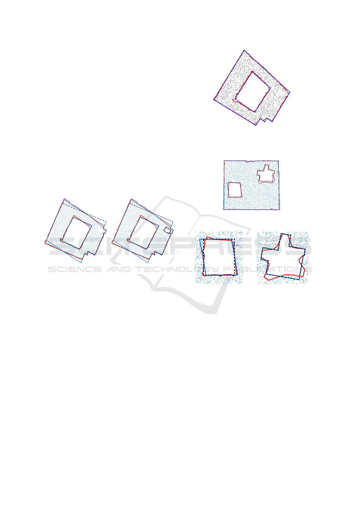
To put our methods for detecting and outlining

holes to the test, we created the synthetic data set de-

picted in Figure 12. The star-shaped hole was man-

ually cropped and is especially challenging, because

it is very sensitive to the choice of k: The edges of

the spires are v-shaped and using large values of k

causes them to become cut off. Using smaller val-

ues of k increases the accuracy, but also increases the

uncertainty for determining the dominant directions

when straightening the outline (see Figures 12(b) and

12(c)). Since we only consider two dominant direc-

tions with this approach, the outline of the star almost

completely loses its initial shape. By means of or-

thogonal projection, we get a more faithful outline of

Figure 11: Inner and outer boundaries obtained by orthog-

onal projection (blue) compared to the concave hull (red) at

k = 20 of our test data set D

. The minimum hole diameter

is d

min

= 50 units.

(a) straightened bound-

aries

(b) straightened lower

left hole boundary

right hole boundary

Figure 12: Outlines created from our approach based on

dominant directions of data set D

compared to the con-

cave hull (red) at k = 20 and k = 40 for the inner and outer

boundaries, respectively. With the star-shaped hole and the

outer boundary, the two dominant directions obtained from

the peaks of the angle histogram (blue) are the same as the

ones obtained by the “90

◦

angle” option (dashed black). In

case of the other hole, the two options yield different domi-

nant directions.

the star-shaped hole, which not perfect, though (see

Figure 13).

GRAPP 2016 - International Conference on Computer Graphics Theory and Applications

Figure 13: Outline of the star-shaped hole in data set D

cre-

ated by orthogonal projection (blue) using k = 10 in com-

parison to the concave hull (red).

5.2 Discussion

The two methods presented in this work for gener-

ating straight outlines have different advantages over

each other. Straightening concave hulls by means

of dominant directions can accurately capture certain

shapes of objects represented by point sets without

prior knowledge about the orientation of their edges.

However, it relies on the prior computation of concave

hulls and is likely to yield unsatisfactory results if the

shape’s edges run in more than two distinct directions

(cf. Figures 10 and 12(c)). Determining the domi-

nant direction is furthermore subject to the width of

bins used for the histogram of angles in the concave

hull. This inﬂuence becomes apparent in Figures 9(c)

and 9(d) where the bin widths are 10

◦

and 1

◦

, respec-

tively. Depending on the quality of the concave hull

(i.e., mainly on the choice of k) and the point distri-

bution, changing the bin width can tilt the generated

outline in an undesirable way. Especially by deter-

mining the second dominant direction from the his-

togram peaks, the choice of bin width may cause a

shift in the position of the peaks corresponding to the

dominant directions. For example, by enlarging the

bin width by 5

◦

, the bin associated with the second

maximum may coincide with a neighboring bin. In

this way, the second direction is tilted by about the

same amount. Of course, the ﬁrst direction can suf-

fer from the same problem, if the point set is of rather

square or circular shape instead of an elongated one.

Our approach based on orthogonal projection and

the dragging of edges can create faithful outlines of

shapes whose edges run in more than two distinct

directions, but it requires hints about the initial ori-

entation of the shape and possibly contained holes.

These hints may be obtained automatically (see Sec-

tion 3.2.3) in some situations, but otherwise they have

to be provided by the user. With this method, it is not

necessary to compute concave hulls or other interme-

diate polygons in advance, though.

The choice of the size k of the neighborhood

considered is crucial for both our methods, but it

is also subject to the distribution of the underlying

points. While the Concave Hull Algorithm starts

at the smallest k = 3 and increases the value if the

outline has self-intersections or does not include all

points of the set, this proceeding is not guaranteed

to succeed with our methods, because our angular

outlines may deliberately exclude points. In our

experiments, we found that using k of about 5 – 10%

of the number of points in the set is a reasonable

initial choice, if the point distribution (excluding

holes to be detected) is approximately uniform.

The decision which outline matches the underly-

Generating Straight Outlines of 2D Point Sets and Holes using Dominant Directions or Orthogonal Projections

ing object “best” is up to the user who can incorporate

background information about the underlying object.

In case of the underlying building represented by D

(see Figures 7 and 8), for instance, we could not de-

cide whether the object is a single building complex

or if there are two separate buildings, possibly linked

by a corridor, if we solely rely on the information pro-

vided by the point set.

6 CONCLUSION AND FUTURE

WORK

In this article, we presented two methods based on

the Concave Hull Algorithm to create straight, angu-

lar and non-convex outlines of 2D point sets and pos-

sibly contained holes. The outlines of point sets rep-

resenting man-made structure, like buildings, created

by means of our methods are “better” than concave

hulls or boundaries obtained from α-shapes to the ef-

fect that our methods capture straight edges more ac-

curately and feature only few, distinct angles.

The employment of straightening concave hulls

by means of dominant directions to generate outlines

is preferable if the orientation of the underlying shape

is unknown or cannot be provided, or if the shape is

known to have edges running in only two distinct di-

rections, e.g., in case of rectangular buildings. Ad-

ditional directions could be obtained by introducing

an angle of tolerance ϕ

max

. If ](e

) > ϕ

max

∀ϕ ∈

{

β,γ

}

, the corresponding label vector entry is set to

zero (see Section 3.1). These edges would not be af-

fected by the straightening procedure, which is help-

ful if the building contains a narrowing or constric-

tions of angles other than the determined dominant

ones.

If information about the orientation of the shape

is available, our approach based on orthogonal pro-

jection can produce more faithful boundary polygons,

especially if the underlying shape features edges run-

ning in more than two distinct directions. More-

over, this approach forgoes the computation of con-

cave hulls or any other intermediate polygon.

The most challenging task is the reliable detection

of holes. We encountered this problem by means of

a heuristic that is subject to sampling problems and

may have several theoretical limitations. Although we

did not encounter major problems due to a rather spe-

ciﬁc, practical application, we would like to improve

on these potential issues. For example, holes might

be located close to the outer boundary of the associ-

ated point set, and they might thus share boundaries

with the exterior outline. This could cause our current

algorithms for bordering holes to fail, because the out-

line might “leave” the hole and intersect the exterior

boundary.

Moreover, we only considered “isolated” point

sets so far. In the application of building reconstruc-

tion, for example, this requires prior segmentation of

the source data. We would like to forgo this step

and determine spacings or gaps between distinct clus-

ters of points in larger point sets to segment these

while creating the corresponding outlines. This may

be accomplished by a combination of modifying and

constraining the neighborhoods employed by our ap-

proaches or the Concave Hull Algorithm, and adjust-

ments of our heuristic for hole detection to this prob-

lem, but remains future work to do.

REFERENCES

Asaeedi, S., Didehvar, F., and Mohades, A. (2013).

Alpha Convex Hull, a Generalization of Convex

Hull. The Computing Research Repository (CoRR),

abs/1309.7829.

Bendels, G. H., Schnabel, R., and Klein, R. (2006). De-

tecting Holes in Point Set Surfaces. Proceedings of

The 14th International Conference in Central Europe

on Computer Graphics, Visualization and Computer

Vision, 14.

de Berg, M., Cheong, O., van Krevald, M., and Overmars,

M. (2008). Computation Geometry. Springer, 3rd edi-

tion.

Douglas, D. and Peucker, T. (1973). Algorithms for the Re-

duction of the Number of Points Required to Repre-

sent a Digitized Line or Its Caricature. The Canadian

Cartographer, 10(2):112 –– 122.

Duckham, M., Kulik, L., Worboys, M., and Galton, A.

(2008). Efﬁcient Generation of Simple Polygons for

Characterizing the Shape of a Set of Points in the

Plane. Pattern Recognition, 41(10):3224–3236.

Edelsbrunner, H., Kirkpatrick, D., and Seidel, R. (1983).

On the Shape of a Set of Points in the Plane. IEEE

Transactions on Information Theory, 29(4):551 – 559.

Galton, A. and Duckham, M. (2006). What is the Region

Occupied by a Set of Points? In Proceedings of the 4th

International Conference on Geographic Information

Science, GIScience’06, pages 81–98, Berlin, Heidel-

berg. Springer-Verlag.

Jarvis, R. A. (1973). On the Identiﬁcation of the Convex

Hull of a Finite Set of Points in the Plane. Information

Processing Letters, 2(1):18 – 21.

Moreira, A. and Santos, M. Y. (2007). Concave hull: A

k-nearest Neighbours Approach for the Computation

of the Region Occupied by a Set of Points. Proceed-

ings of the 2nd International Conference on Computer

Graphics Theory and Applications (GRAPP), pages

61 – 68.

Ramer, U. (1972). An Iterative Procedure for the Polygonal

Approximation of Plane Curves. Computer Graphics

and Image Processing, 1(3):244 – 256.

GRAPP 2016 - International Conference on Computer Graphics Theory and Applications

Vosselman, G. (1999). Building Reconstruction Using Pla-

nar Faces In Very High Density Height Data. In Inter-

national Archives of Photogrammetry, Remote Sens-

ing and Spatial Information Sciences, pages 87–92.

Wang, J. and Oliveira, M. M. (2007). Filling Holes on

Locally Smooth Surfaces Reconstructed from Point

Clouds. Image and Vision Computing, 25(1):103 –

113.

Wang, O., Lodha, S. K., and Helmbold, D. P. (2006). A

Bayesian Approach to Building Footprint Extraction

from Aerial LIDAR Data. In Proceedings of the Third

International Symposium on 3D Data Processing, Vi-

sualization, and Transmission (3DPVT’06), 3DPVT

’06, pages 192–199, Washington, DC, USA. IEEE

Computer Society.

Wu, X. and Chen, W. (2014). A Scattered Point Set

Hole-ﬁlling Method Based on Boundary Extension

and Convergence. In 11th World Congress on Intel-

ligent Control and Automation, pages 5329 – 5334.

IEEE.

Generating Straight Outlines of 2D Point Sets and Holes using Dominant Directions or Orthogonal Projections