
Structural Synthesis based on PCA: Methodology and Evaluation
Sriniwas Chowdhary Maddukuri
2
, Wolfgang Heidl
1
, Christian Eitzinger
1
and Andreas Pichler
2
1
Department of Machine Vision, Profactor GmbH, Im Stadtgut A2, Steyr-Gleink, Austria
2
Department of Robotics and Assistive Systems, Profactor GmbH, Steyr-Gleink, Austria
Keywords: Structural Synthesis, Surface Inspection, Decision Boundary, Principal Components Analysis, Elastic Net
Regularization.
Abstract: In recent surface inspections systems, interactive training of fault classification is becoming state of the art.
While being most informative for both training and explanation, fault samples at the decision boundary are
rare in production datasets. Therefore, augmenting the dataset with synthesized samples at the decision
boundary could greatly accelerate the training procedure. Traditionally, synthesis methods had proven to be
useful for computer graphics applications and have only been applied for generating samples with stochastic
and regular texture patterns. Presently, the state of the art synthesis methods assume that the test sample is
available and are feature independent. In the context of surface inspection systems, incoming samples are
often classified to several defect classes after the feature extraction stage. Therefore, the goal in this
research work is to perform the synthesis for a new feature vector such that the resulting synthesized image
visualizes the decision boundary. This paper presents a methodology for structural synthesis based on
principal components analysis. The methodology expects the samples of the training set as an input. It
renders the synthesized form of the input samples of training set through eigenimages and its computed
coefficients by solving a linear regression problem. The methodology has been evaluated on an industrial
dataset to validate its performance.
1 INTRODUCTION
Synthesis is defined as the process of generating a
sample which is close to the visual appearance of the
input sample. In the context of surface inspection
systems, synthesis plays a vital role in rendering
fault instances that lie on the decision boundary.
Assuming the surface inspection system is
embedded with a dynamic classifier. The dynamic
classifier uses the extracted features of the incoming
samples and performs the classification to existing
or new defect classes. The dynamic classifier
updates the decision boundary through which it
communicates its decision to the end-users (i.e.
machine operators).
Communicating classifier decision to end-users
often requires the synthesis of fault instances to
visualize the decision boundary between classes.
This led to the motivation of generating synthesized
images which are located either close to or on the
decision boundary within the n-dimensional feature
space. Therefore, a methodology for structural
synthesis based on principal components analysis is
presented in this research work.
1.1 Related Work
In general, synthesis methods assumes that the test
sample is available where small patch region is
obtained from it and then synthesized to render a
sample of arbitrary size with texture similar to that
of the test sample or fill the missing regions of the
test sample. Parametric texture synthesis methods
explicitly measure some set of statistics in the input
sample in an analysis step. In the synthesis step, an
arbitrary image (e.g. initialized with random noise)
is altered according to constraints derived from the
previously extracted statistics. (Heeger and Bergen,
1995) uses a random noise image which is modified
to match filter response histograms, obtained at
different scales in the analysis step. Good results for
stochastic textures were reported, but the method
failed to capture structured or regular texture
patterns. More recently (Portilla and Simoncelli,
2000) proposed a texture synthesis method based on
350
Maddukuri, S., Heidl, W., Eitzinger, C. and Pichler, A.
Structural Synthesis based on PCA: Methodology and Evaluation.
DOI: 10.5220/0005721403480355
In Proceedings of the 11th Joint Conference on Computer Vision, Imaging and Computer Graphics Theory and Applications (VISIGRAPP 2016) - Volume 3: VISAPP, pages 350-357
ISBN: 978-989-758-175-5
Copyright
c
2016 by SCITEPRESS – Science and Technology Publications, Lda. All rights reserved

the first and second order statistics of joint wavelet
coefficients. Similar to Heeger and Bergen, these
coefficients are obtained for different scales of the
input texture. While the synthesis quality for regular
textures could be improved, this approach still lacks
capabilities to reproduce structured textures. The
major advantage of parametric texture synthesis
methods is that the statistics of the synthesized
image can be explicitly controlled. For this reason
parametric texture synthesis is highly relevant for
experimental design in the field of human perception
(Balas, 2006) (Balas et al., 2009). All parametric
texture synthesis approaches share the disadvantage,
that several iterations are required until the multi-
scale representation of the output texture is altered to
match the statistics of the input sample. This
optimization process is time consuming, in particular
when compared to pixel based or patch based
synthesis methods (Moore and Lopes, 1999).
Current pixel-based synthesis methods are based
on (Efros and Leung, 1999) which follow a very
simple idea. Starting from an input exemplar, the
output is first initialized by copying a small seed
region from the input. The synthesized region is then
gradually grown from the initial seed by assigning
the output pixels one by one in an inside-out, onion
layer fashion. The colour of each output pixel is
determined by a neighbourhood searching for
similar neighbourhoods in the input image. From
this candidate set of matching neighbourhoods the
output pixel is chosen from the centre of a randomly
selected neighbourhood from the candidate set. This
process is repeated until all the output pixels are
assigned. In order to speed up this process, the
search for matching neighbourhoods (Wei and
Levoy, 2000) may be made more efficient using tree
search (Kwatra et al., 2005), jump-maps (Zelinka
and Garland, 2004) or k-coherence (Tong et al.,
2002); (Thumfart, 2012).
Restoring of structure in image with
missing/damaged regions is investigated e.g. in (Guo
et al., 2008) using morphological erosion and
structure feature replication or (Chen and Xu, 2010)
which builds upon a primal sketch representation
model for the reconstruction of missing structure. In
contrast to (Guo et al., 2008), the methodology
presented here describes the use of eigenimages to
synthesize the test sample. In the absence of test
sample, the proposed methodology tries to restore
the structure of the test sample using the
neighbouring samples which are either close to or on
the decision boundary. Therefore, the principal
components analysis approach of utilizing the
eigenimages was more suitable for our application.
1.2 Paper Organization
Section 2 describes the methodology for structural
synthesis. Section 3 will explain the evaluation
procedure, simulation setup and its results will be
discussed. A few details about the dataset on which
the evaluation procedure was performed will also be
given in Section 3. Section 4 concludes the research
work and provides an outlook regarding the future
work.
2 METHODOLOGY
The methodology proposed in this section focuses
on the structural synthesis of classified images. The
methodology assumes the following pre-requisites to
be fulfilled for performing structural synthesis:
Acquire a training set of classified images
Resize the training set images with constant
width and height
Extracted features of the training set images must
be available
2.1 Principal Components Analysis
Principal components analysis (PCA) is one of the
methods applied for dimensionality reduction of a
dataset while retaining most of the information in
the dataset. The principal components analysis
method is based on the following assumptions:
Dimensionality of the dataset can be efficiently
reduced by linear transformation
Information of the dataset is concentrated in
those directions where input data variance is
maximum
Assume ‘N’ number of resized images are contained
in the training set. Every resized image I(x, y) is a
matrix of size n x n of 8-bit gray scale intensity
values. Initially, the training set images are formed
into a single rectangular matrix
of size n
2
x N.
⋯
(1)
Using Eq. (1) as an input, eigenimages are then
computed by applying the PCA method (Belhumeur,
Hespanha, and Kriegman, 1997). The result of
principal components method is given by Eq. (2).
(2)
where , and represent eigenimages matrix,
score matrix and eigenvalues vector respectively. In
the next step, images are projected onto the subspace
Structural Synthesis based on PCA: Methodology and Evaluation
351

of eigenimages to compute the coefficient matrix
(Turk and Pentland, 1991). The subspace of
eigenimages is selected from the number of non-zero
elements contained in the eigenvalues vector. The
coefficient matrix is represented by Eq. (3) and Eq.
(4).
μ
(3)
…
,
(4)
where ,
and μ represent coefficient matrix,
subspace of eigenimages and column wise mean of
respectively. m corresponds to the number of
non-zero elements of . The subspace of the
coefficient matrix is dependent upon the selection of
desired number of eigenimages in
. The selection
of desired number of eigenimages in
is given by
Eq. (5).
, 01
(5)
where
and represent the scalar parameters
responsible for deriving the subspace of coefficient
matrix. The preferable choice for parameter should
be close to its higher limit (Noortiawati et al., 2006).
The subspace of coefficient matrix and the desired
number of eigenimages in
are represented by Eq.
(6) and Eq. (7).
⊆
…
,
(6)
⊆
…
(7)
where
and
represent the subspace of
coefficient matrix and desired number of
eigenimages respectively.
and
are then
applied in the later stages of the methodology for
synthesizing an image for a given new feature
vector. In the subsequent section, solving of linear
regression problem of C
s
will be described.
2.2 Linear Regression
Linear regression is a statistical approach for
modelling the behaviour of dependent variables
denoted by Y and independent variables denoted by
X. Here, the subspace of coefficient matrix C
s
resulting from the Section 2.1 is considered as the
subspace of the dependent variable Y and the
Feature matrix is considered as the independent
variable X. A linear regression model is assumed to
fit the dependent variable Y. The linear regression
model is represented by Eq. (8).
(8)
where β is the parameter matrix. , and are
represented by Eqs. (9) – (11).
1
,
⋯
,
1
,
⋯
,
⋮
1
⋮
,
⋱
⋯
⋮
,
(9)
,
,
,
⋮
,
,
⋮
,
⋯
,
⋯
⋱
⋯
,
⋮
,
⋮
⋮
(10)
,
,
⋯
,
,
,
⋯
,
⋮
,
⋮
,
⋱
⋯
⋮
,
(11)
where a and b represent the original width and
height of the resized images of the training set. In
the first instance, least squares method was applied
to estimate the parameter matrix β. The least squares
method seeks to minimize the sum of squared
residual errors
.
min
∈
(12)
where
and
represent the column vectors of
matrices and respectively. The unique solution
for the estimate of parameter vector
is given by
the Eq. (13).
(13)
To avoid overfitting situations where the ratio of
model complexity to the training set size is too high,
Elastic Net regularization method is chosen (Hastie
et al., 2001). Elastic Net regularization method
solves the cost function represented in Eqs. (14) –
(16).
min
∈
1
2
(14)
1
2
.
‖
‖
‖
‖
(15)
0, 01
(16)
where is the complexity parameter. The publicly
available package glmnet (Qian et al., 2013) is
applied for estimating the parameter vector
.
Assuming N images are available with the training
set. Let’s say N-1 images are used in the training
phase for computing l number of solutions in λ for
estimating
and k
th
image which is left out in the
VISAPP 2016 - International Conference on Computer Vision Theory and Applications
352
training phase is used for validation phase (Friedman
et al., 2010). During the validation phase, a measure
risk (i.e. absolute error) is computed for each value
of . Then, the where the measure risk is minimal
will be selected and its resulting parameter vector
is chosen. In the subsequent section, synthesizing of
images for new feature vectors will be described.
2.3 Synthesis
Synthesizing an image for a given new feature
vector
is generated using the estimated parameter
matrix
from Section 2.2 and the desired number of
eigenimages EI
rs
from Section 2.1. Initially, a
dependent variable is derived for generating new
coefficient vector and estimating the size of the
synthesized image. The new dependent variable
and the resultant coefficient vector
are
represented by Eq. (17) and Eq. (18).
(17)
,
1
(18)
Finally, the synthesized image I
syn
is obtained from
the matrix multiplication of EI
rs
and c
w
.
(19)
The synthesized image is reshaped back to an image
of n x n size. This reshaped image is then resized
using the estimated width and height which can be
retrieved as the last two entities of the new
dependent variable
.
3 EVALUATION
In this section, the evaluation procedure of the
proposed methodology will be explained in detail. A
few details about the dataset on which the evaluation
was done will be mentioned. The simulation setup
and subsequent results will also be presented here.
3.1 Sheaves Dataset
The inspected sheaves with a diameter of around
100mm are applied in wire rope-based elevators. It
comprises a steel wheel body coated with
polyurethane on the circumference that carries the
rope notch. Coating is exercised through a casting
process with the final notch shape produced in a
turning lathe. The following are the event types of
the inspected sheaves:
Type 1: Surface spots that occurred during
lathing also known as lathing damages
Type 2: Events detected by the segmentation
processes that do not correspond to surface faults
also known as false positives from segmentation
Type 3: Delamination of the coatings
Type 4: Closed cavities
Type 5: Open cavities
Type 6: Swarf (turnings) that adhere to the
circumference
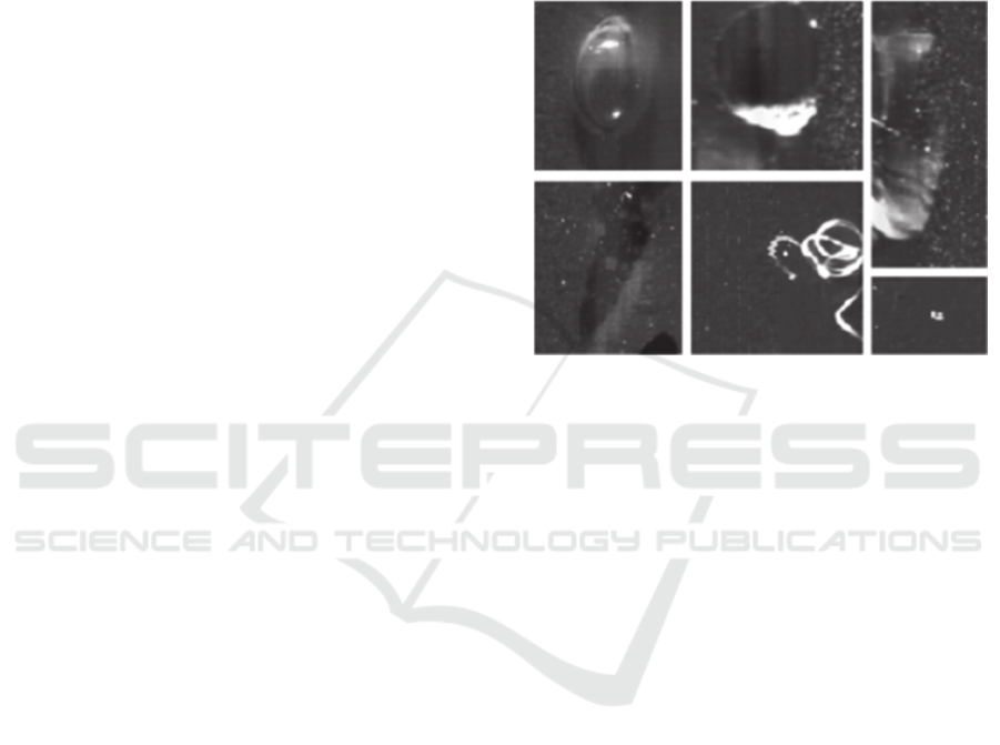
Figure 1: Examples of event types on elevator sheaves.
Row-wise, left-to-right: closed cavities, open cavities,
lathing damages, delamination, swarf, false positives from
segmentation.
Typical examples of aforementioned event types
are shown in Figure 1 (Weigl et al., 2014).
Inspection of the sheaves is confined to the coated
circumference which is scanned by a line-scan
camera with a resolution of 20µm per pixel.
Classification of event types which were detected on
the elevator sheaves is performed using a random
forest classifier. The classifier is trained on a fully
expert-annotated database. The output of the
classifier consists of the extracted feature vectors
and class probability vectors of the respective
images. The features computed for the images which
correspond to the event types describe the shape,
size, intensity level, histograms of the events.
3.2 Simulation Setup
Given 6 classes of Sheaves dataset, there will be 15
unique possible class pairs. For a given class pair
(CP), images are selected in such a way that the first
two highest class probabilities present in their
respective class probability vector are close to each
other. The steps for acquiring the training set images
for all class pairs are the following:
Step 1: Class probabilities present in the class
probability vector of all the images of Sheaves
Structural Synthesis based on PCA: Methodology and Evaluation
353
dataset are sorted in ascending order
Step 2: Gradient between the first two highest
class probabilities using the sorted class
probability vector from step 1 is computed
Step 3: Five percent of the maximum class
probability is assigned as a threshold value. This
threshold value is then compared with the
gradient from step 2 for selecting specific images
from the dataset which belong to the 15 class
pairs
Step 4: Assuming the evaluation procedure has
been initiated for a given class pair. Then, the
images resulting from step 3 for the given class
pair are sorted in such a way that the gradient
(computed from step 2) values are in ascending
order
Step 5: The sorted out images from step 4 are
then used as the training set for the given class
pair
Except for ‘delamination/open cavities’,
‘delamination/swarf’ and ‘closed cavities/swarf’
class pairs, images close to the decision boundary
for the remaining 12 class pairs were found with
respect to the above selection procedure.
Let’s assume ‘N’ test samples (i.e. images) are
contained in the training set of j
th
class pair and each
test sample is of different size. For evaluation, we
are holding out the i
th
instance (test sample) from the
training set and this one instance is then synthesized.
Likewise, this process is repeated for all N number
of instances in the training set.
Synthesized form of the test samples resulted
from the evaluation are then fed to feature extraction
software for computing their respective feature
vectors.
3.3 Results
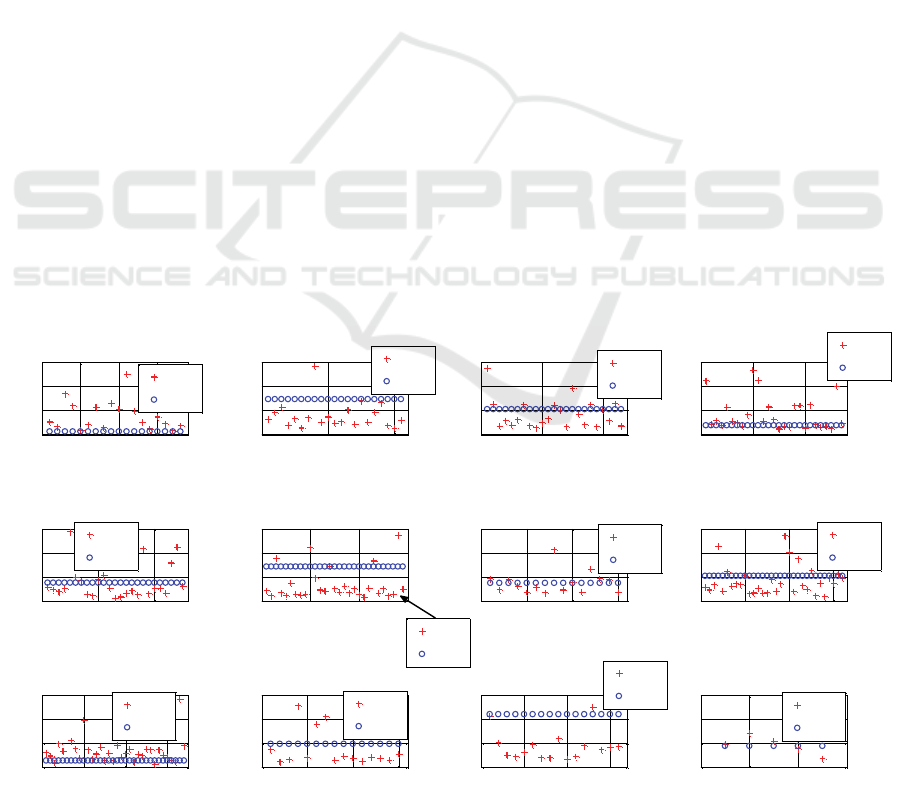
In this section, the evaluation results will be
discussed. Figure 2 represents the Euclidean distance
‘ED
r,s
’ computed between feature vectors of the test
samples (i.e. training set of j
th
class pair) and that of
the synthesized form of test samples. Here, the
distance between the feature vectors of the k
th
test
sample with the highest probability indicating that it
belongs to the first class and l
th
test sample with the
highest probability indicating that it belongs to the
second class of the training set of j
th
class pair is
considered as the performance metric. This
performance metric is denoted by ‘Ed
om
’ in Figure 2.
Assuming an ideal scenario where the computed
euclidean distance is close to zero, this will give an
indication that the synthesized form of test samples
are a close approximation of the test samples in
terms of feature vectors and visual appearance. Here,
the evaluation result is far from the ideal scenario.
However, euclidean distance of majority of the
synthesized form of test samples of ‘lathing
damages/delamination’, ‘lathing damages/closed
cavities’, ‘lathing damages/swarf’, ‘false positives
from segmentation/delamination’, ‘false positives
from segmentation/closed cavities’, ‘false positives
Figure 2: Euclidean distance versus index of synthesized test samples of feasible 12 class pairs.
0 5 10 15
0
5
10
15
index of synthesized image
Euclidean distance
CP:lathing damages
/false positives from segmentation
ED
r,s
ED
om
0 10 20
0
5
10
15
index of synthesized image
Euclidean distance
CP:lathing damages
/delamination
ED
r,s
ED
om
0 10 20
0
5
10
15
index of synthesized image
Euclidean distance
CP:lathing damages
/closed cavities
ED
r,s
ED
om
0 10 20
0
5
10
15
index of synthesized image
Euclidean distance
CP:lathing damages
/open cavities
ED
r,s
ED
om
0 10 20
0
5
10
15
index of synthesized image
Euclidean distance
CP:lathing damages
/swarf
ED
r,s
ED
om
0 10 20 30
0
5
10
15
index of synthesized image
Euclidean distance
CP:false positives from segmentation
/delamination
ED
r,s
ED
om
0 5 10 15
0
5
10
15
index of synthesized image
Euclidean distance
CP:false positives from segmentation
/closed cavities
ED
r,s
ED
om
0 10 20 30
0
5
10
15
index of synthesized image
Euclidean distance
CP:false positives from segmentation
/open cavities
ED
r,s
ED
om
0 10 20 30
0
5
10
15
index of synthesized image
Euclidean distance
CP:false positives from segmentation
/swarf
ED
r,s
ED
om
0 5 10 15
0
5
10
15
index of synthesized image
Euclidean distance
CP:delamination
/closed cavities
ED
r,s
ED
om
0 5 10 15
0
5
10
15
index of synthesized image
Euclidean distance
CP:closed cavities
/open cavities
ED
r,s
ED
om
0 2 4 6
0
5
10
15
index of synthesized image
Euclidean distance
CP:open cavities
/swarf
ED
r,s
ED
om
VISAPP 2016 - International Conference on Computer Vision Theory and Applications
354
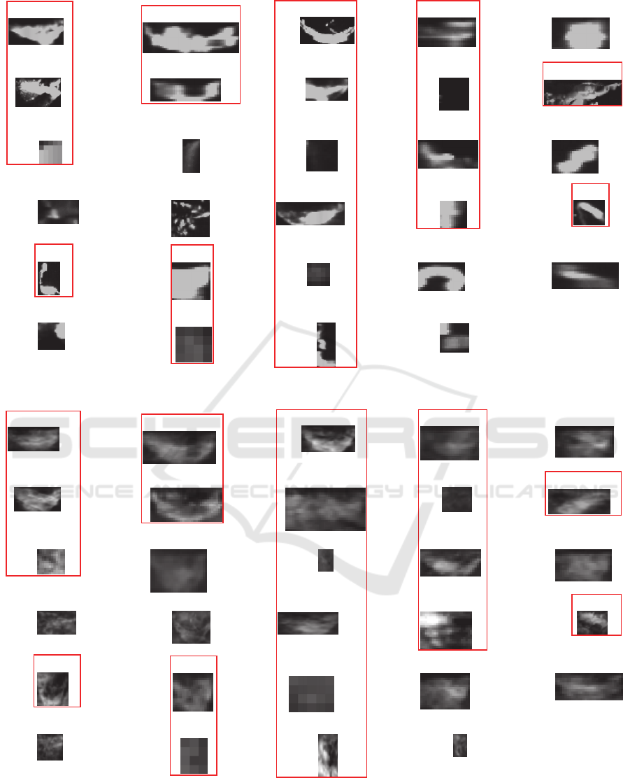
Figure 3: Test samples of ‘lathing damages/open cavities’ class pair.
Figure 4: Synthesized form of test samples of the ‘lathing damages/open cavities’ class pair.
from segmentation/open cavities’,
‘delamination/closed cavities’ and
‘delamination/open cavities’ class pairs are within
their respective performance metric value. This
gives an indication that those synthesized form of
test samples lie within the hypersphere (formed by
Im: 1
Im: 2
Im: 3 Im: 4 Im: 5
Im: 6 Im: 7 Im: 8 Im: 9
Im: 10
Im: 11 Im: 12 Im: 13 Im: 14 Im: 15
Im: 16 Im: 17
Im: 18
Im: 19 Im: 20
Im: 21 Im: 22 Im: 23 Im: 24 Im: 25
Im: 26 Im: 27 Im: 28 Im: 29
Syn Im: 1
Syn Im: 2
Syn Im: 3 Syn Im: 4 Syn Im: 5
Syn Im: 6 Syn Im: 7 Syn Im: 8 Syn Im: 9
Syn Im: 10
Syn Im: 11 Syn Im: 12 Syn Im: 13 Syn Im: 14 Syn Im: 15
Syn Im: 16 Syn Im: 17
Syn Im: 18
Syn Im: 19 Syn Im: 20
Syn Im: 21 Syn Im: 22 Syn Im: 23 Syn Im: 24 Syn Im: 25
Syn Im: 26 Syn Im: 27 Syn Im: 28 Syn Im: 29
Structural Synthesis based on PCA: Methodology and Evaluation
355

the test samples located as points in n-dimensional
feature space) in which the corresponding test
samples are contained.
For the remaining class pairs, the synthesized
images are located away from the hypersphere in
which the corresponding test samples are comprised.
This is due to the fact that, each and every image
present in the training set of these class pairs is very
distinct in shape and structure. Nevertheless, an
average of 58.5% of the synthesized images resulted
from all 12 class pairs are within the average of the
performance metrics of all 12 class pairs.
Figures 3 and 4 represent the test samples and
the synthesized form of test samples of ‘lathing
damages/open cavities’ class pair respectively. From
Figures 3 and 4, it can be seen that the methodology
performs the synthesis of specific test samples
(which are shown in the red rectangular boxes)
reasonably well. The cause behind such result is the
structure and shape present in the i
th
specific test
sample is still visible from the remaining samples of
‘lathing damages/open cavities’ class pair and are
contained as the prominent principal components in
the eigenimage matrix at PCA stage. Therefore,
more than half of the synthesized samples (i.e.
synthesized form of test samples) are close to the
test samples in terms of visual appearance. Similarly
for the remaining class pairs, the number of
synthesized samples which were visually close with
their respective test samples was found to be approx.
in between 50% to 60%.
4 CONCLUSION
A methodology for performing structural synthesis
based on principal components analysis is
formulated here. Also, a framework for the feature
based synthesis evaluation procedure has been
presented. The methodology has been evaluated on a
dataset from elevator sheaves inspection. Test
samples on which the methodology performs the
synthesis quite good is shown with respect to a
certain class pair. Although satisfactory result was
obtained for the remaining class pairs where test
samples were fewer, the methodology might have
worked better if the class pairs consisted of high
number of test samples. In contract to state of the art
texture and structural synthesis methods which
assumes the availability of a test sample, the
proposed methodology is able to generate
synthesized form of the test sample using the
neighbouring samples which lie close to the decision
boundary. This enables an inspection system’s
human operator to visualize the decision boundary
where availability of test samples lying close to the
decision boundary is rare. The next step in this
research work is to enhance the PCA with kernel
functions to compute principal components in high-
dimensional space, related to the input space by
some nonlinear map. In addition, we intend to factor
the dominant fault orientation out of the principal
component decomposition in a similar way varying
fault sizes are handled now. Using a subspace of
these principal components, the linear regression and
synthesis steps from the methodology could be
repeated to acquire much better visual closeness of
the synthesized samples with that of test samples.
ACKNOWLEDGEMENTS
This research work was funded via the projects
‘Improving the usability of machine learning in
industrial inspection systems’ (useML, Grant
number: 840202) and ‘Generating process feedback
from heterogeneous data sources in quality control’
(Grant number: 849962) by the Austrian Research
Promotion Agency (FFG) under the scope of the
‘Information and communication technology of the
future’ program. This program is promoted by the
Austrian Federal Ministry of Transport, Innovation
and Technology (BMVIT) and the Federal Ministry
of Science, Research and Economy (BMWFW). It
reflects only the authors’ views.
REFERENCES
Heeger, D.J., Bergen, J.R., Moore, R., 1995. Pyramid-
based texture analysis/synthesis. In SIGGRAPH’95,
Proceedings of the 22
nd
Annual Conference on
Computer Graphics and Interactive Techniques, pp.
229–238, New York, USA.
Portilla, J., Simoncelli, E.P., 2000. A Parametric Texture
Model Based on Joint Statistics of Complex Wavelet
Coefficients. International Journal of Computer
Vision – Special issues on Statistical and
Computational Theories of Vision: Modelling,
learning, sampling and computing, vol. 40, issue 1,
pp. 49–70.
Balsa, B.J., 2006. Texture synthesis and perception: Using
computational models to study texture representations
in the human visual system. Vision Research, vol. 46,
issue 3, pp. 299–309, PERGAMON.
Balas, B.J., Nakano, L., Rosenholtz, R., 2009. A
summary-statistic representation in peripheral vision
explains visual crowding. Journal of Vision, vol. 9,
issue 12, pp. 1–18.
VISAPP 2016 - International Conference on Computer Vision Theory and Applications
356

Efros, A. A., Leung, T.K., “Texture synthesis by non-
parametric sampling”, in Computer Vision, 1999. The
Proceedings of the Seventh IEEE International
Conference on, vol. 2, no., pp. 1033–1038, 1999.
Wei, L.-Y., Levoy, M., 2000. Fast texture synthesis using
tree-structures vector quantization. In SIGGRAPH’00,
Proceedings of the 27
th
Annual Conference on
Computer Graphics and Interactive Techniques, pp.
479–488.
Kwatra, V., Essa, I., Bobick, K.A., Kwatra, N., 2005.
Texture optimization for example-based synthesis. In
SIGGRAPH’05, Proceedings of ACM SIGGRAPH
2005, vol. 24, issue 3. pp. 795–802.
Zelinka, S., Garland, M., 2004. Jump map-based
interactive texture synthesis. ACM Transactions on
Graphics, vol. 23, issue 4, pp. 930–962.
Tong, X., Zhang, J., Liu, L., Wang, X., Shum, H.-Y, 2002.
Synthesis of bidirectional texture functions on
arbitrary surfaces. In SIGGRAPH’02, Proceedings of
ACM SIGGRAPH 2002, vol. 21, issue 3, pp. 665–672.
Thumfart, S., “PhD Thesis: Genetic Texture Synthesis”,
Johannes Kepler University Linz, Department of
Computational Perception, 2012.
Guo, H., Ono, N., Sagayama, S., 2008. A Structure-
Synthesis Image Inpainting Algorithm based on
Morphological Erosion Operation. In CISP’08,
Proceedings of the 2008 Congress on Image and
Signal Processing, vol. 3, issue 27 – 30, pp. 530 – 535.
Xiaowu, Chen., Fang, Xu., 2010. Automatic Image
Inpainting by Heuristic Texture and Structure
Completion. In MMM’10, Proceedings of the 16
th
International Conference on Advances in Multimedia
Modelling, pp. 110 – 119.
Belhumeur, P.N., Hespanha, J.P., Kriegman, D.,
“Eigenfaces vs Fisherfaces: Recognition Using Class
Specific Linear Projection”, in Pattern Analysis and
Machine Intelligence, IEEE Transactions on, vol. 19,
no. 7, pp. 711–720, July 1997.
Turk, M., Pentland, A.P., “Face recognition using
eigenfaces”, in Computer Vision and Pattern
Recognition, 1991. IEEE Computer Society
Conference on, vol., no., pp. 586–591, 3–6 June 1991.
Noortiawati, T. M. D., Hussain, A., Samad, S.A., Hussain,
H., Marzuki, M. M., 2006. Eigenposture for
Classification. Journal of Applied Science, vol. 6,
issue 2, pp. 419–424.
Hastie, T., Tibshirani, R., Friedman, J., 2001. The
Elements of Statistical Learning, Springer New York
Inc., New York, 2
nd
edition.
Friedman, J., Tibshirani, R., Hastie, T., 2010.
Regularization paths for generalized linear models via
coordinate descent. Journal of Statistical Software.
vol. 33, no. 1, URL: http://www.jstatsoft.org/v33/i01.
Qian, J., Hastie, T., Friedman, J., Tibshirani, R., Simon,
N., 2013. Glmnet for Matlab. URL:
http://www.stanford.edu/~hastie/glmnet_matlab/
Weigl, E., Heidl, W., Lughofer, E., Radauer, T., Eitzinger,
C., 2014. On Improving Performance of Surface
Inspection Systems by On-line Active Learning and
Flexible Classifier Updates. In MACH VISION
APPL’14, Machine Vision and Applications. Springer-
Verlag.
Structural Synthesis based on PCA: Methodology and Evaluation
357
