Motion based Segmentation for Robot Vision using Adapted

EM Algorithm

Wei Zhao and Nico Roos

Department of Knowledge Engineering, Maastricht University, Maastricht, The Netherlands

Keywords:

Optical Flow, SIFT Matching, Clustering, Motion Segmentation.

Abstract:

Robots operate in a dynamic world in which objects are often moving. The movement of objects may help

the robot to segment the objects from the background. The result of the segmentation can subsequently be

used to identify the objects. This paper investigates the possibility of segmenting objects of interest from the

background for the purpose of identiﬁcation based on motion. It focusses on two approaches to represent the

movements: one based on optical ﬂow estimation and the other based on the SIFT-features. The segmentation

is based on the expectation-maximization algorithm. A support vector machine, which classiﬁes the segmented

objects, is used to evaluate the result of the segmentation.

1 INTRODUCTION

Studies of visual perception show that human vision

is based on seeing changes (Martinez-Conde et al.,

2004). In the domain of robot vision, seeing changes

also crucial because of the environments are mostly

dynamic: robots operate in a dynamically chang-

ing world and they may have the capability to move

around. We will investigate applicability of detecting

changes in robot vision in this paper.

Analysing the changes among the frames can give

us a clue of objects in the video (Karasulu and Ko-

rukoglu, 2013; Zappella et al., 2008). This is called

the moving object detection, which is differs from the

objects detection in single image. Detecting an object

in single image requires knowledge about object’s ex-

pressions.

In this paper, a general system is investigated to

detect and recognize the objects by their movements.

We assume that one object consists of a group of

points, and points belong to the same object will have

the same movement. The system consists of three

main steps. Firstly, we detect all points and their

movements in the video sequences, where two meth-

ods are investigated. One uses optical ﬂow to estimate

the motions of all pixels of an image. The other uses

higher level features, e.g. the scale-invariant feature

transform (or SIFT) points. Secondly, the points are

segmented into different groups based on their move-

ments and scales. These groups of points are possible

objects. Segmentation of these points based on their

movement is fulﬁlled by combining the EM algorithm

with a divisive hierarchical approach. Finally, a sup-

port vector machine (SVM) (Boser et al., 1992) is

used to evaluate the whether the segmentation results

can be recognized accurately as an object.

In the next section, we will brieﬂy review some re-

lated work. Section 3, provides some background in-

formation about the algorithms that we have applied.

Section 4 outlines our approach. Experiments that we

used to evaluate our approach are presented in Section

5. Section 6 concludes the paper.

2 RELATED WORK

Detecting objects from images is multi-purpose tasks,

where many techniques, such as images segmenta-

tion, image processing, machine learning, linear al-

gebra, statistic, etc., are involved in.

Much research has already been done in the area

of image segmentation. A high level division of the

available techniques are: detecting discontinuities and

detecting similarities (Narkhede, 2013). The ﬁrst cat-

egory uses edge detection to identify regional bound-

aries (Narkhede, 2013). The second category consists

of techniques such as: thresholding, clustering, mo-

tion segmentation and color segmentation (Seerha and

Rajneet, 2013; Narkhede, 2013).

In this paper we focus on motion segmentation.

Motion segmentation using optical ﬂow and k-means

Zhao, W. and Roos, N.

Motion based Segmentation for Robot Vision using Adapted EM Algorithm.

DOI: 10.5220/0005721606490656

In Proceedings of the 11th Joint Conference on Computer Vision, Imaging and Computer Graphics Theory and Applications (VISIGRAPP 2016) - Volume 3: VISAPP, pages 651-658

ISBN: 978-989-758-175-5

651

clustering has been proposed by (Wang and Adelson,

1994). Borshukov et al. (Borshukov et al., 1997) im-

proved this method by replacing the k-means cluster-

ing with a multistage merging step clustering. Opti-

cal ﬂow estimation in combination with the EM algo-

rithm for the purpose of image stabilization has been

proposed by (Pan and Ngo, 2005).

(Shi and Malik, 1998) proposed a motion segmen-

tation algorithm that constructs a weighted spatio-

temporal graph on image sequence and using normal

cuts to ﬁnd the most salient partitions of the spatio-

temporal graph. (Weiss, 1997) presented an algorithm

that segments the image sequences by ﬁtting the mul-

tiple smooth ﬂow ﬁelds to the spatio-temporal data

using a variant of the EM algorithm.

We make use of the basic principles of the men-

tioned approaches: detecting the motion ﬁelds and

segmenting them into clusters using EM algorithm.

But our work differs from previous work in several

ways. First, the objects need not to be cut perfectly,

just sufﬁciently consistent to enable object identiﬁca-

tion. Secondly, the descriptions of clusters are simple

and improved gradually.

3 PRELIMINARIES

The approach proposed in this paper makes use of

optical ﬂow estimation (OFE), scale-invariant fea-

ture transform (SIFT), the expectation-maximization

(EM) algorithm and the support vector machine

(SVM). In this section we brieﬂy review each of these

approaches.

3.1 Optical Flow Estimation

Optical ﬂow estimation is deﬁned as the distribution

of apparent velocities of movement of brightness pat-

terns in an image (Horn and Schunck, 1981). The

optical ﬂow Estimation is based on the assumption

that the intensity of a pixel corresponding with a point

on an object, does not change when the object or the

camera is moving. Suppose the location of a point is

(x, y) at time t and (x + ∆x, y + ∆y) at time t + ∆t. Let

I(x, y, t) be the intensity of a pixel w.r.t position (x, y)

and time t. Based on the assumption of brightness

constancy, i.e.,

I(x + ∆x, y + ∆y,t +∆t) = I(x, y,t) (1)

Expanding the equation with ﬁrst-order Taylor series,

and using the notation (u, v) = (

), we get:

∇I(x, y,t) · (u, v, 1)

= 0 (2)

Lucas and Kanade(Lucas et al., 1981) proposed an

additional assumption that the that neighboring pix-

els often have the same movement. Given the set

of neighbouring points, the optical ﬂow of centroid

points of the neighbourhood is able to estimated by

solving the optimized problem of Equation 2 over

these neighbouring points.

3.2 Scale-Invariant Feature Transform

SIFT is an algorithm to detect and describe local fea-

tures in images, which was proposed by David Lowe

(Lowe, 1999). Unlike the optical ﬂow, SIFT is not

a technique for detecting changes. SIFT feature de-

scriptors are some keypoints extracted from a set of

reference images. They are invariant to image scaling

and rotation, and partially invariant to afﬁne distor-

tion, noise and illumination changes. Because of the

scale-invariant properties and the high level feature

expression, the movement of segments in the image

can be estimated by matching the keypoints between

two successive images.

3.3 Expectation-Maximization

Algorithm

Both OFE and SIFT can provide motion vectors of

point in an image. We assume that points belonging to

one object have motion vectors that can be described

by an afﬁne transformation. To extract the object

from the background, clustering methods are needed

to cluster points of these objects. It is also a segmen-

tation task, which aims to segment the image into ob-

jects and background based on the motion features

of pixels or points. The Expectation-Maximization

(EM) algorithm is one of the approaches enables us

to do this.

The EM algorithm (Dempster et al., 1977) is an

effective and popular technique for estimating pa-

rameters of a distribution from a given data set. It

aims at determining the most likely values of param-

eters θ using observed data x and some hidden vari-

ables Z. That is, the most likely parameters θ max-

imizes the expected expected value of the likelihood

L(θ;x, Z) = P(x, Z | θ) over all hidden variables Z, so,

θ = argmax

L(θ

;x)

where: L(θ;x) = P(x | θ) =

∑

P(x, Z | θ)

(3)

Equation 3 is a ﬁxed point equation. Given the pa-

rameters θ and x we can determine the probability dis-

tribution of the hidden variables Z, and subsequently

we can ﬁnd a maximum likelihood estimate of the pa-

rameters θ. The former is called the expectation step

VISAPP 2016 - International Conference on Computer Vision Theory and Applications

652

Motion

Estimation

clustering

Filtering

SVM

classifer

Recognition

results

Image

sequence

Object

...

Segmented

images

Figure 1: Basic architecture of the detection and recognition approach.

while the latter is called the maximization step. Start-

ing from an initial estimate of θ or P(x, Z | θ) and re-

peatedly applying the expectation and maximization

step, the EM algorithm will converge to the maximum

likelihood parameters θ.

Instead of the probability distribution P(x, Z | θ)

we may determine:

z = argmax

P(x, Z | θ) (4)

in the expectation step. In the maximization step we

determine:

θ = argmax

L(θ

;x, z) (5)

4 MOTION-BASED VISION

Although this paper focusses on segmentation, the ﬁ-

nal goal is the identiﬁcation of objects a robot is see-

ing in the world. The results of the segmentation

should be evaluated with respect to this goal. There-

fore we will present the whole architecture (Figure 1)

of the vision system, including the classiﬁcation of

observed objects.

4.1 Optical Flow based Motion

Detection

The optical ﬂow is calculated by using the iterative

Lucas-Kanade method with pyramids in this system

(Bouguet, 2001). The pyramid optical ﬂow estima-

tion allows a high accuracy when the displacements

are not too large. However, optical ﬂow estimation

often fails to estimate the large displacement due to

the constant brightness assumption.

The optical ﬂow computes the displacement of ev-

ery pixels, so the pixels are selected as points. To

improve the computational efﬁciency, we resized the

images to the resolution of 120*160.

4.2 SIFT based Motion Detection

To deal with large movements, we adopt the scale-

invariant feature transform (SIFT) to detect the scale-

invariant features. The movements of SIFT features

can be identiﬁed by matching the corresponding fea-

tures of two frames (Lowe, 2004).

The SIFT algorithm ﬁrst detects the location of the

keypoints in two frames separately, then compute the

SIFT descriptor for each keypoint, which is a 128 di-

mensional feature vector (Lowe, 1999). Keypoints

between two images can be matched by using the

nearest-neighbours approach. The Euclidean distance

between two SIFT feature vectors is used to evaluate

the similarity of vectors. A SIFT feature vector D

is matched to a SIFT feature D

only if the distance

satisfy the following two conditions:

• The distance is smaller than some threshold.

• The distance is not greater than the distance of D

to all other descriptors.

For the ﬁrst condition, the ratios between the distance

of the nearest neighbor and the second nearest neigh-

bour are calculated. According to Lowe’s research

(Lowe, 2004), the matches are accepted in which the

distance ratio is smaller than 0.8, which will result in a

highest accuracy of matching. However, the matched

results may still include some incorrect matches due

to the imprecision of the SIFT model. RANSAC (Fis-

chler and Bolles, 1981) is used to reﬁne the matching

by ﬁltering out the “bad” matches.

A pair of matched vectors denotes the geometric

information of the same keypoint in two different im-

ages. The movement vector of such keypoint can be

obtained by computing the displacement of the coor-

dinates. We can generate a ﬂow ﬁeld by computing

the movement vectors for all matched keypoints.

4.3 Parametric Motion Model of

Moving Object

Both the optical ﬂow and SIFT matching can produce

a set of movement vectors to denote the geometric

transformations of relevant points. The movement of

one object can be a combination of a translation, a ro-

tation and a scaling. In other words, an afﬁne transfor-

mation (AF) can be used to denote the movement of

an object. Assuming that objects will not change their

shapes, i.e. the same object looks almost the same in

all frames of the sequence, we assume that the dis-

placement of all points in this object will satisfy the

afﬁne transformation.

Motion based Segmentation for Robot Vision using Adapted EM Algorithm

653

Let x = (x, y)

the position of one point in a frame,

and let x

= (x

, y

)

be the position of corresponding

point in the next frame. This pair (x, x

) indicates the

movement of one point between 2 frames. Then

= Ax + b;

(6)

where A =





, b =





The six afﬁne transformation parameters of (A, b)

form the parametric motion model of the object.

4.4 Motion based Segmentation

Motion-based segmentation aims to group together

the points with the same movement. Since points be-

longing one object will have the same movement, we

may use the movement to identify the points that be-

long to one object. An afﬁne model with six parame-

ters is used to indicate the movement of an object. We

use modiﬁed EM algorithm with a recursive division

strategy to determine the clusters of points; i.e., the

segmentations.

Algorithm 1 gives the main steps of the EM based

segmentation algorithm. Each group of points in this

algorithm indicates an object.

Algorithm 1: EM-based segmentation algorithm.

Set the number of objects to 1;

Put all points into one group;

repeat

Calculate the parameters (A, b) of the afﬁne

transformation of each group of points (see

Equation 7);

Reassign each point to a group (determine the

value of variable z) based on the error of the

point w.r.t. each group;

until convergence

if the group with the largest errors given the

group parameters (A, b) exceeds the threshold

then

Split the group with the largest errors;

Increase the number of objects by 1;

end if

until no group can be ﬁnd to split, or a maximum

number of iterarions reached.

There are four key components in this algorithm,

• How to determine the parameters (A, b) of the

afﬁne transformation?

• How to determine the best assignment of points

for each group?

• How to determine the group to be split?

• How to split the group?

Given a group of points and their locations in

two frames, we can obtain the afﬁne parameters by

solving Equation 6. In practice, the groups could

contain outliers because the segmentation is not per-

fectly. The parametric motion model (A, b) of the

afﬁne transformation of a group G is obtained by solv-

ing the optimization problem:

(A, b) = argmin

(A,b)

∑

(x,x

)∈G

||ε||

subject to ε = x

− Ax − b

(7)

Suppose there are K groups, the division of points

is regarded as an optimization problem:

min

∑

k∈[1,...,K]

(8)

where E

∑

(x,x

)∈G

||ε||

Given a partition of points, each group has an

average error

with respect to its motion

model (A, b)

. The group with largest average errors

is selected to be split, while the largest error is marked

as the error of current partition. The selected group

can be split into 2 sub-groups using a bisecting K-

means algorithm (Selim and Ismail, 1984). Then the

number of groups is increased by 1 and a new parti-

tion of the points is computed by solving Equation 8.

If the error of the new partition is smaller than the er-

ror of the old partition, the current partition is updated

by using the new partition and motion model. Other-

wise, it means the optimal partition is found and no

groups is able to be split, i.e. the iteration comes to an

end.

4.5 Segmentation of Sequences

Section 4.4 describe the segmentation based on the

movement between two frames. To extend the seg-

mentation to sequences, we need to make use of the

historical information. A probability matrix P

N×K

built to indicate the probabilities of each point with

regards to each group. Here N denotes the number of

points and K is the number of groups. Given a par-

tition (G

, G

, ...G

), the probability of point i with

regard to group k is estimated:

i,k

= 1 −

i,k

∑

j=1

i, j

+ δ

(9)

where δ = 0.1, which is used for preventing divided

by zero. The EM segmentation computes such a prob-

ability matrix for each pair of successive frames. If a

point presents in F successively frames, the trajectory

VISAPP 2016 - International Conference on Computer Vision Theory and Applications

654

of movement vectors has a length of F − 1. The prob-

ability of points w.r.t. the sequence is a combination of

the probability computed from last frame pair and the

historical probabilities as shown in Equation 10. In

Equation 10, the parameter α is a factor to decrease

the weight of historical data, which is set as 0.85 in

the experiments.

p(i, k|v

, v

< f

) =

p(i, k|v

) + αp(i, k|v

< f

)

1 + α

(10)

Note that unlike other segmentation algorithms

(Shi and Malik, 1998; Borshukov et al., 1997; Elham-

ifar and Vidal, 2009), we do not require that points are

present in all frames.

4.6 Classiﬁcation

The previous stages results in a segmented image,

which separates the moving objects with different

movement. For the optical ﬂow based segmenta-

tion, the detected regions are groups of pixels, which

means the image is divided in to small image patches.

SIFT based segmentation result in groups of SIFT fea-

tures. So in the classiﬁcation stage, we need to deal

with 2 kinds of input data, the pixel level images and

the bags of SIFT features.

A Support Vector Machine with an RBF kernel is

chosen to fulﬁll the classiﬁcation task in this paper.

5 EXPERIMENT

The approach proposed in this paper gives an archi-

tecture for detecting and recognizing moving objects

from videos. The main component of our approach is

the task of motion segmentation. Thus, we will eval-

uated our approaches in the following ways:

• Evaluate object detection results, with Optical

ﬂow based and SIFT based motion segmentation

respectively.

• Compare the segmentation results using our

method with some control approaches.

• Test the quality of classiﬁcations (recognition)

when using the result of the segmentation as in-

put.

The segmentation is evaluated on video sequences

from three database: the robocup 2014 video

, CNnet

2014 (Wang et al., 2014) and the Hopkins155 motion

database

. Figure 2 shows some instances of the im-

ages from different sequences. The classiﬁcation of

https://www.youtube.com/watch?v=dhooVgC 0eY

http://www.vision.jhu.edu/data/hopkins155/

segmented images is evaluated on results of all above

segmentations.

5.1 Objects Detection in Videos

Our approach is examined on the 20 videos mentioned

above, whose composition is described in Table1.

Table 1: The composition of tested videos containing dif-

ferent number of objects.

Number of videos

Number of Objects

Camera

2 3 2-3 2-4

CNnet2014 2 3 2 3 ﬁxed

Robocup 3 2 3 2 moving

For each video clip which has a frame rate of 24

to 30 fps , a sequence of 30 frames is selected for

test. To compare the motion detection results using

optical ﬂow and SIFT matching, we tested the ac-

curacy of segmentation results using different frame

rates. That is, new sequences are generated from each

sequence by selecting frames with an interval of itv

(where itv = 3, 5, 10), while the original sequence has

itv = 1. For the sequences with larger intervals, the

displacement of points between two frames increases.

The movement of a point is represented by its co-

ordinates in two neighbouring frames, thus there is a

set of points X

∈ R

2×N

for frames f = 1, ...F, where

is the number of feature points detected in frame

f . For the OFE motion detection N

is ﬁxed for all

frames, which is 120 × 160. For the SIFT detection,

trajectories are discontinuous for SIFT points, where

varies from 300 to 500 for different frames.

Table 2 shows accuracy of segmentation results

with different intervals of sequences.

Table 2: The average accuracy (%) of segmentation us-

ing our approach, with different intervals, based on the 20

videos (from CNnet2014 and robocup competition video).

(a) Test with optical ﬂow based motion

Number of objects

Interval of frames

1 3 5 10

2 88.2 85.4 78.2 63.6

3 91.0 82.0 81.3 61.6

2-3 79.6 73.2 65.1 59.0

2-4 76.9 69.4 60.1 58.2

all 83.9 77.5 71.2 60.6

(b) Test with SIFT based motion

Number of objects

Interval of frames

1 3 5 10

2 97.8 99.5 98.3 97.4

3 98.0 96.9 99.0 98.6

2-3 94.9 99.8 98.2 80.0

2-4 96.7 98.9 92.0 74.1

all 96.9 98.8 96.9 87.5

Motion based Segmentation for Robot Vision using Adapted EM Algorithm

655

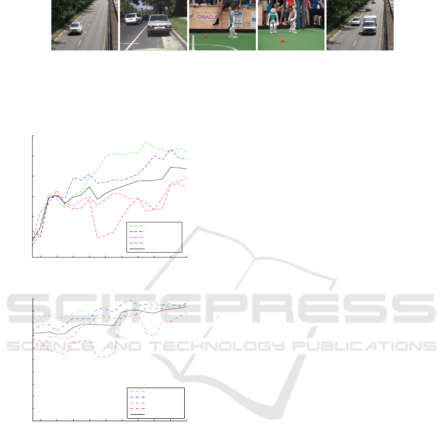
Figure 2: Images from test sequences.

Figure 3a and Figure 3b show the curves of aver-

age accuracy of motion segmentation with regards to

the number of frames that have been processed. Here

itv = 1.

Index of frames

2 4 6 8 10 12 14 16 18 20

Accuracy(%) of segmentation using OFE

100

fixed 2 objects

fixed 3 objects

varied from 2 to 3

varied from 2 to 4

all

(a) optical ﬂow based motion segmentation

2 4 6 8 10 12 14 16 18 20

100

Index of frames

Accuracy(%) of segmentation using SIFT motions

fixed 2 objects

fixed 3 objects

varied from 2 to 3

varied from 2 to 4

all

Videos of

(b) SIFT based motion segmentation

Figure 3: Accuracy curves w.g.t. the index of frames, using

(a) Optical ﬂow based motions and (b) SIFT based motions.

The red line indicates the average accuracy of all video se-

quences in test. The slash line indicates the average accu-

racy over sequence with different number of objects, which

are drawn with different colors.

From the result, we can make the following conclu-

sions:

1. SIFT based motion segmentation performs bet-

ter than optical ﬂow based method in 2 ways.

Firstly The number of points of SIFT detection

are smaller, which requires for less computational

resources. Secondly, the accuracy of SIFT based

segmentation is always higher than optical ﬂow.

2. For the sequences with changing number of ob-

jects, the accuracy ﬂuctuates at the frames where

the number of objects changes. Despite the

changing number of objects, both methods show

an general increasing trend in segmentation accu-

racy.

3. The approach can deal with ﬁxed number of ob-

jects as well as changing number of objects, with

a maximum of 4 objects in the test. The per-

formance of segmentation with changing number

of objects is slightly worse than the test with ﬁx

number of objects.

5.2 Comparison of Motion

Segmentation

In this section, a comparison test is described based

on the database of Hopkins155, which contains of 155

videos of 29 or 30 frames, each contains 2 or 3 mov-

ing objects. The trajectories of feature points are pro-

vided by the database (the average number of feature

points is 266 for 2 objects, while it’s 398 for 3 ob-

jects). Only the segmentation part of our approach

is evaluated in this section. The objects of “checker-

board” make 3D rotations and translations. The “traf-

ﬁc” sequences contain moving vehicles of outdoor

trafﬁc scene. The remaining sequences named “artic-

ulated” contain motions constrained by joints, head

and face motions, people walking, etc. Over half of

the videos are taken using a moving camera.

Our segmentation method named as adapted EM

segmentation for motion sequences (AEMS), is com-

pared with the SSC (Elhamifar and Vidal, 2009), LSA

(Yan and Pollefeys, 2006), RANSAC (Fischler and

Bolles, 1981), and ALC (Rao et al., 2008). Table

3 shows the segmentation accuracy for sequences of

Hopkins155, Table 4 shows the accuracy of ﬁnding

the number of objects in sequence for AEMS.

The SCC outperforms all methods in general. The

performance of our approach varies for categories.

On average, our method ranks 3rd out of 5 methods.

We can also draw the conclusion from the results:

1. AEM performs with a high accuracy of 99% when

there are only 2-dimension translations.

2. AEM is sensitive to 3-dimensions rotation and

scaling.

3. AEM can ﬁnd the number of objects automati-

cally, with a high accuracy of 96.2%.

VISAPP 2016 - International Conference on Computer Vision Theory and Applications

656

Table 3: Accuracy (%) of motion segmentation using dif-

ferent methods.

(a) sequences with 2 motions.

LSA RANSAC ALC SSC AEMS

Checkerboard:78 sequences

97.4 93.5 98.5 98.8 93.4

Trafﬁc:31 sequences

94.6 97.4 98.4 99.9 99.4

Articulated: 11 sequences

95.9 92.7 89.3 99.4 93.2

All: 120 sequences

96.0 94.5 95.4 99.4 95.3

(b) sequences with 3 motions.

LSA RANSAC ALC SSC AEMS

Checkerboard:26 sequences

94.2 74.2 94.8 97.0 86.6

Trafﬁc:7 sequences

74.9 87.2 92.3 99.4 99.1

Articulated: 2 sequences

92.8 78.6 78.9 98.6 79.6

All: 35 sequences

87.3 80.0 88.7 98.3 88.4

LSA RANSAC ALC SSC AEMS

All:155 sequences

91.6 87.3 92.0 98.8 91.9

Table 4: Accuracy (%) of estimating the number of objects.

Number

of objects

Checker-board Trafﬁc Articulated

2 92.8 96.6 81.2

3 86.7 98.4 83.6

all 89.9

4. The AEM methods is not affected by the camera

with a 2-dimensional movement, since the video

sequences used in the experiment are taken using

a ﬁxed or a moving camera.

Note that the comparative methods require trajec-

tories with ﬁxed dimensions, as well as with a ﬁxed

number of moving objects. In contrast, our method is

able to handle changing numbers of objects, and fea-

ture points that presented in only a part of a trajectory.

5.3 Classiﬁcation

The result of motion segmentation provides groups

of points, each of which should represent one object.

The next step is to recognize the objects. We classify

the segmented results using a SVM classiﬁer. There

are two types of segmentation results in section 5.1:

1. optical ﬂow based method provides image frac-

tions because points are pixels from image;

2. SIFT based methods gives the groups of SIFT

points, each point is associated with a feature vec-

tor. The groups of SIFT features are coded into

vectors of the same dimension using the bag of

word methods (Csurka et al., 2004).

The sequences contain 8 categories of objects, includ-

ing cube, conical frustum, curved paper, car, truck,

robot, pedestrian, face. We used a training set con-

tains 80 sequences from the total 20 + 155 sequences

for training and the rest for testing.

The classiﬁcation results of the 8 categorises are

listed in Table 5a. Table 5b shows the classiﬁcation

results of only for cars and trucks, using a classiﬁer

that was trained with a different database namely Cal-

tech256

The results indicate that, segmentation accuracy

is sufﬁcient to recognize the objects, for the database

tested.

6 CONCLUSIONS

In this paper we proposed an architecture for mov-

ing object detection and recognition in video se-

quences based on detecting changes and clustering

movements. We compared two approaches for de-

tecting objects motions. One is based on optical ﬂow

motion detection which detect the changes between

pixels. The other is based on SIFT which detect the

SIFT points and ﬁnd the motions by matching points

between frames. An adapted EM algorithm is used

to cluster the moving points, which gives us the seg-

mentation. An SVM is used to identify the segmented

objects.

The results shows that higher level-feature (SIFT)

has the advantage of a lower computation time and a

higher accuracy in segmentation. The main character-

istic of our methods has the ability to handle a chang-

ing set of feature points. Because of the objects move-

ments, feature points may not be visible in all frames.

Moreover, our method can determine the number of

objects. Experiment shows that our method perform

especially well for the 2D movement.

In the future work, we need to evaluate our method

on sequences with more than 4 objects. An extension

to a 3D motion model is also needed for applications

in robot vision. Last but not least, more research is

needed with regard to the other methods of feature

detecting and motion extraction.

http://authors.library.caltech.edu/7694/

Motion based Segmentation for Robot Vision using Adapted EM Algorithm

657

Table 5: Accuracy (%) of classiﬁcation using SVM.

(a) All sequences

robots cars trucks pedestrian Conical cube cylinder face

OFE 78 92 100 72 98 93 96 98

SIFT 82 89 66 75 95 95 97 99

(b) “cars” and “trucks”

cars trucks

OFE 97.9 98.5

SIFT 97.2 96.9

REFERENCES

Borshukov, G. D., Bozdagi, G., Altunbasak, Y., and Tekalp,

A. M. (1997). Motion segmentation by multi-stage

afﬁne classiﬁcation. IEEE Trans. Image Processing,

6:1591–1594.

Boser, B. E., Guyon, I. M., and Vapnik, V. N. (1992). A

training algorithm for optimal margin classiﬁers. In

Proceedings of the ﬁfth annual workshop on Compu-

tational learning theory, pages 144–152. ACM.

Bouguet, J.-Y. (2001). Pyramidal implementation of the

afﬁne lucas kanade feature tracker description of the

algorithm. Intel Corporation, 5.

Csurka, G., Dance, C., Fan, L., Willamowski, J., and Bray,

C. (2004). Visual categorization with bags of key-

points. In Workshop on statistical learning in com-

puter vision, ECCV, volume 1, pages 1–2. Prague.

Dempster, A. P., Laird, N. M., and Rubin, D. B. (1977).

Maximum likelihood from incomplete data via the em

algorithm. Journal of the Royal Statistical Society. Se-

ries B (Methodological), pages 1–38.

Elhamifar, E. and Vidal, R. (2009). Sparse subspace clus-

tering. In Computer Vision and Pattern Recognition,

2009. CVPR 2009. IEEE Conference on, pages 2790–

2797. IEEE.

Fischler, M. A. and Bolles, R. C. (1981). Random sample

consensus: a paradigm for model ﬁtting with appli-

cations to image analysis and automated cartography.

Communications of the ACM, 24(6):381–395.

Horn, B. K. and Schunck, B. G. (1981). Determining optical

ﬂow. In 1981 Technical Symposium East, pages 319–

331. International Society for Optics and Photonics.

Karasulu, B. and Korukoglu, S. (2013). Moving object de-

tection and tracking in videos. In Performance Evalu-

ation Software, pages 7–30. Springer.

Lowe, D. G. (1999). Object recognition from local scale-

invariant features. In Computer vision, 1999. The pro-

ceedings of the seventh IEEE international conference

on, volume 2, pages 1150–1157. Ieee.

Lowe, D. G. (2004). Distinctive image features from scale-

invariant keypoints. International journal of computer

vision, 60(2):91–110.

Lucas, B. D., Kanade, T., et al. (1981). An iterative image

registration technique with an application to stereo vi-

sion. In IJCAI, volume 81, pages 674–679.

Martinez-Conde, S., Macknik, S. L., and Hubel, D. H.

(2004). The role of ﬁxational eye movements in vi-

sual perception. Nature Neuroscience, 5:229 – 240.

Narkhede, H. (2013). Review of image segmentation tech-

niques. International Journal of Science and Modern

Engineering (IJISME), 1:5461.

Pan, Z. and Ngo, C.-W. (2005). Selective object stabiliza-

tion for home video consumers. IEEE Trans. Con-

sumer Electronics, 51(4):1074–1084.

Rao, S. R., Tron, R., Vidal, R., and Ma, Y. (2008). Mo-

tion segmentation via robust subspace separation in

the presence of outlying, incomplete, or corrupted tra-

jectories. In Computer Vision and Pattern Recogni-

tion, 2008. CVPR 2008. IEEE Conference on, pages

1–8. IEEE.

Seerha, G. K. and Rajneet, K. (2013). Review on recent

image segmentation techniques. International Jour-

nal on Computer Science and Engineering (IJCSE),

5:109–112.

Selim, S. Z. and Ismail, M. A. (1984). K-means-type algo-

rithms: a generalized convergence theorem and char-

acterization of local optimality. Pattern Analysis and

Machine Intelligence, IEEE Transactions on, (1):81–

87.

Shi, J. and Malik, J. (1998). Motion segmentation and track-

ing using normalized cuts. In Computer Vision, 1998.

Sixth International Conference on, pages 1154–1160.

IEEE.

Wang, J. Y. and Adelson, E. H. (1994). Representing

moving images with layers. Image Processing, IEEE

Transactions on, 3(5):625–638.

Wang, Y., Jodoin, P.-M., Porikli, F., Konrad, J., Benezeth,

Y., and Ishwar, P. (2014). Cdnet 2014: An expanded

change detection benchmark dataset. In Computer Vi-

sion and Pattern Recognition Workshops (CVPRW),

2014 IEEE Conference on, pages 393–400. IEEE.

Weiss, Y. (1997). Smoothness in layers: Motion segmenta-

tion using nonparametric mixture estimation. In Com-

puter Vision and Pattern Recognition, 1997. Proceed-

ings., 1997 IEEE Computer Society Conference on,

pages 520–526. IEEE.

Yan, J. and Pollefeys, M. (2006). A general framework for

motion segmentation: Independent, articulated, rigid,

non-rigid, degenerate and non-degenerate. In Com-

puter Vision–ECCV 2006, pages 94–106. Springer.

Zappella, L., Llad

o, X., and Salvi, J. (2008). Motion seg-

mentation: a review. In Proceedings of the 2008 con-

ference on Artiﬁcial Intelligence Research and Devel-

opment: Proceedings of the 11th International Con-

ference of the Catalan Association for Artiﬁcial Intel-

ligence, pages 398–407. IOS Press.

VISAPP 2016 - International Conference on Computer Vision Theory and Applications

658