
Parameter Estimation for HOSVD-based Approximation of Temporally
Coherent Mesh Sequences
Michał Romaszewski and Przemysław Głomb
Institute of Theoretical and Applied Informatics, Polish Academy of Sciences, Bałtycka 5, 44-100, Gliwice, Poland
Keywords:
3D Animation, Compression, TCMS, HOSVD, Decomposition, Approximation.
Abstract:
This paper is focused on the problem of parameter selection for approximation of animated 3D meshes (Tem-
porally Coherent Mesh Sequences, TCMS) using Higher Order Singular Value Decomposition (HOSVD). The
main application of this approximation is data compression. Traditionally, the approximation was done using
matrix decomposition, but recently proposed tensor methods (e.g. HOSVD) promise to be more effective.
However, the parameter selection for tensor-based methods is more complex and difficult than for matrix de-
composition. We focus on the key parameter, the value of N-rank, which has major impact on data reduction
rate and approximation error. We present the effect of N-rank choice on approximation performance in the
form of rate-distortion curve. We show how to quickly create this curve by estimating the reconstruction error
resulting from the N-rank approximation of TCMS data. We also inspect the reliability of created estima-
tor. Application of proposed method improves performance of practical application of HOSVD for TCMS
approximation.
1 INTRODUCTION
Three-dimensional meshes are one of the most com-
mon representations of a virtual surface with applica-
tions in computer simulations, entertainment, medical
imaging and digital heritage documentation. Com-
plexity of processing, visualization and storage of
modelled objects resulted in the rapid development
of methods for mesh compression, as summarised in
(Maglo et al., 2015).
Particularly interesting group of methods is re-
lated to compression of temporally coherent mesh se-
quences (TCMS), also called dynamic animations or
animated meshes, well defined in (Arcila et al., 2013).
TCMS is a sequence of meshes ordered in time, with
a constant number of vertices, connectivity and topol-
ogy. One particularly successful approach to TCMS
compression employs Principal Component Analysis
(PCA). The general idea was presented in (Alexa and
Muller, 2000). The animation was converted to a ma-
trix by stacking meshes frame-by-frame. Authors rep-
resented each frame of the animation as a linear com-
bination of principal components, obtained through
decomposition of the animation matrix. Such repre-
sentation allows to transmit only a limited number of
first principal components and efficiently reconstruct
the original sequence with limited distortion. Further
works refined this idea, e.g. the COBRA algorithm
described in (V
´
a
ˇ
sa and Skala, 2009) reaches compres-
sion ratio between 0.5 and 5 bit per frame per ver-
tex (bpfv) for a KG error (a measure commonly used
to compare TCMS compression algorithms and de-
scribed in (Karni and Gotsman, 2004)) of 0.05%.
As an alternative to matrix approximation, TCMS
data can be expressed in the form of a mode-3 ten-
sor T and tensor decomposition may be employed.
One particularly suitable method is the Higher Order
Singular Value Decomposition (HOSVD), described
in detail in (Kolda and Bader, 2009). Its recent ap-
plication to data compression was presented e.g. in
(Ballester-Ripoll and Pajarola, 2015).
HOSVD transforms the mode-3 TCMS tensor T
into the Tucker operator (TO). The TO consist of the
core tensor C and three orthogonal factor matrices.
The key property of this representation is the approxi-
mation. The energy of the core tensor is concentrated
in the frontal-upper-left corner so large magnitudes
correspond to its low indices. The TO can be trun-
cated by zeroing the low-index elements, forming a
truncated Tucker operator (TTO). Original data can
be reconstructed from the TTO with the reconstruc-
tion error expressed in the form of tensor Frobenius
norm as ||T −T
0
||.
When applied to TCMS data, HOSVD may al-
140
Romaszewski, M. and Głomb, P.
Parameter Estimation for HOSVD-based Approximation of Temporally Coherent Mesh Sequences.
DOI: 10.5220/0005723501380145
In Proceedings of the 11th Joint Conference on Computer Vision, Imaging and Computer Graphics Theory and Applications (VISIGRAPP 2016) - Volume 3: VISAPP, pages 140-147
ISBN: 978-989-758-175-5
Copyright
c
2016 by SCITEPRESS – Science and Technology Publications, Lda. All rights reserved

low to reach higher data reduction ratio with lower
distortion than PCA, as presented in (Romaszewski
et al., 2013), where authors compare HOSVD and
PCA applied to lossy reconstruction of TCMS se-
quences. They present the performance of these meth-
ods in terms of data size and reconstruction error for
a set of well-known, representative sequences.
The main challenge, hovewer, when applying
HOSVD for TCMS compression lies in finding the
N-rank value to minimize the TTO size with an ac-
ceptable reconstruction error. Usually (e.g. in (Ro-
maszewski et al., 2013)) this is done by searching
through the parameter space. Since the reconstruc-
tion of T from TTO is computationally expensive, the
questions arise: how to estimate the reconstruction er-
ror associated with the specific N-rank, how to find its
optimal value and how reliable is such estimation for
TCMS data?
This paper concentrates on the problem of N-
rank estimation for approximating TCMS data with
HOSVD. The distortion resulting from approximation
is expressed in the form of KG error, commonly used
to compare TCMS compression methods. We show
how to use the estimator to graphically represent the
effect of HOSVD reconstruction in the form of a rate-
distortion curve. We also discuss the estimation relia-
bility using a set of well-known TCMS samples.
The article is organised as follows. The introduc-
tion and related work are presented in Section 1. Def-
initions and methodology are presented in Section 2.
Results are presented in Section 3, while conclusions
can be found in Section 4.
2 METHODOLOGY
Our goal is to estimate the error associated with the N-
rank approximation of the TCMS tensor T using the
HOSVD algorithm. We use this estimation to form
the rate-distortion curve based on N-rank TTO trun-
cation.
2.1 Input Data
Our input data is the temporally coherent mesh se-
quence (TCMS), described in detail in (Arcila et al.,
2013). Such sequence consists of meshes with con-
stant connectivity and varying positions of vertices
in time. We consider only the vertex position data,
since it has the most significant impact on animation
volume. Animation vertices can be represented as a
sequence of F matrices M
k
∈ R
K×J
. The rows of
M
k
are positions of mesh vertices v
i
∈ R
J
, 0 ≤ i < K.
These matrices can form a tensor T = t
i, j,k
∈ R
K,J,F
by stacking M
k
as frontal slices T
::k
, using the nota-
tion from (Kolda and Bader, 2009). In our experi-
ments vertex features are the standard euclidean coor-
dinates only, therefore J = 3.
2.2 Higher Order Singular Value
Decomposition
Higher Order Singular Value Decomposition is a gen-
eralisation of SVD from matrices to tensors. Based
on description provided in (Romaszewski et al., 2013)
and following the conventions presented in (Kolda
and Bader, 2009), HOSVD can be explained in the
following way:
A tensor
T = {t
i
1
,i
2
,...,i
n
}
I
1
−1,I
2
−1,...,I
N
−1
i
1
,i
2
,...,i
n
=0
∈ R
I
1
,I
2
,...,I
N
(1)
has N modes. Each of the indices corresponds to one
of the modes i.e. i
l
to mode l.
By multiplication of tensor T by matrix U =
{u
i
l
d
}
I
l
−1,D
i
l
,d=0
∈ R
I
l
,D
in mode l we define tensor T
0
∈
R
I
1
,...,I
l−1
,D,I
l+1
,...,I
N
, such that:
T
0
= (T ×
l
U)
i
1
...i
l−1
d i
l+1
...i
N
=
I
l
−1
∑
i
l
=0
t
i
1
i
2
...i
l
...i
N
u
i
l
d
.
(2)
By unfolding tensor T in mode l we define matrix
T
(l)
such that
(T
(l)
)
i, j
= t
i
1
...i
l−1
j i
l+1
...i
N
, (3)
where i = 1 +
∑
N
k=1
l6=l
(i
k
− 1)J
k
and J
k
=
∏
k−1
m=1
m6=l
I
m
.
Given tensor T , defined as in Eq. (1), a new sub-
tensor T
i
n
=α
can be created according to the equation
with the following elements:
T
i
l
=α
= {t
i
1
i
2
...i
l−1
i
l+1
...i
n
}
I
1
−1,I
2
−1,...,α,...,I
N
−1
i
1
=0,i
2
=0,...,i
l
=α,...,i
n
=0
(4)
where
T
i
l
=α
∈ R
I
1
,I
2
,...,1,...,I
N
. (5)
The scalar product hA,Bi of tensors A, B ∈
R
I
1
,I
2
,...,I
N
is defined as
hA, Bi =
I
1
−1
∑
i
1
=0
I
2
−1
∑
i
2
=0
. . .
I
N
−1
∑
i
N
=0
b
i
1
,i
2
,...,i
n
a
i
1
,i
2
,...,i
n
. (6)
We say that if scalar product of tensors equals zero,
then they are orthogonal.
The Frobenius norm of tensor T is given by
||T || =
p
hT , T i.
Given tensor T , in order to find its HOSVD,
in the form of the so called Tucker operator
JC ;U
(1)
, . . . , U
(N)
K, such that C ∈ R
I
1
,...,I
N
and U
(k)
∈
R
I
k
,I
k
are orthogonal matrices, Algorithm 1 can be
used.
Parameter Estimation for HOSVD-based Approximation of Temporally Coherent Mesh Sequences
141

Tensor C is called the core tensor and has the fol-
lowing useful properties. Reconstruction: T = C ×
1
U
(1)
×
2
U
(2)
×
3
. . . ×
N
U
(N)
, where U
(i)
are orthogo-
nal matrices. Orthogonality: hC
i
l
=α
, C
i
l
=β
i = 0 for all
possible values of l, α and β, such that α 6= β. Or-
der of sub-tensor norms: ||C
i
n
=1
|| ≤ ||C
i
n
=2
|| ≤ . . . ≤
||C
i
n
=I
n
|| for all n.
Input: Data Tensor T
Output: Tucker operator JC; U
(1)
, . . . , U
(N)
K
for k ∈ {1, . . . , N} do
U
(k)
=
left singular vectors of T
(k)
in unfolding k;
end
C = T ×
1
U
(1)T
. . . ×
N
U
(N)T
;
return JC; U
(1)
, . . . , U
(N)
K;
Algorithm 1: HOSVD algorithm uset to find the
Tucker operator from the tensor T .
Therefore, informally, one can say that larger
magnitudes of a core tensor are denoted by low values
of indices. To explain the HOSVD approximation we
will define the tensor
˜
T =
˜
C ×
1
˜
U
(1)
×
2
˜
U
(2)
×
3
. . . ×
N
˜
U
(N)
, (7)
where
˜
C = {c
i
1
,i
2
,...,i
n
}
R
1
−1,R
2
−1,...,R
N
−1
i
1
,i
2
,...,i
n
=0
∈ R
R
1
,R
2
,...,R
N
(8)
is a truncated tensor in such a way that in each mode l
indices span from 0 to R
l
−1 ≤ I
l
−1 and
˜
U
(l)
∈ R
R
l
,I
l
matrices whose columns are orthonormal and rows
form orthonormal basis in respective vector spaces.
Given (R
l
)
N
l=1
we say that
˜
T approximates T in the
sense of their euclidean distance ||
˜
T − T ||.
2.3 Estimation of Reconstruction Error
One way of finding the optimal (given the error
threshold) N-rank value for the data tensor T , is to
perform multiple reconstructions of T from TTO. Un-
fortunately, such search is time consuming. It could
be, however, avoided with a reliable estimator of the
N-rank reconstruction error. Our task is therefore to
define the reconstruction error metric, to find an esti-
mator, and to assess its reliability.
2.3.1 The Metric for Reconstruction Error
We argue that the most useful error metrics for the
TCMS reconstruction estimator would be the distor-
tion measure used to compare TCMS compression al-
gorithms, namely the KG error. The KG error was
defined in (Karni and Gotsman, 2004) to express the
distortion of TCMS compression based on PCA. Its
benefit is that it allows to compare the distortion in-
troduced by HOSVD-based approximation with the
final results of state-of-art TCMS compression algo-
rithms. It should be noted, however, that KG error
does not correlate well with perceptual distortion of
animations and its shortcomings were noted e.g. in
(V
´
a
ˇ
sa and Skala, 2009). Since the KG error was origi-
nally defined using matrix operations, we will express
it using the tensor notation in the following way:
Given tensor T = t
i, j,k
∈ R
K,J,F
we define the
average trajectory tensor E(T ) = e
i, j,k
∈ R
K,J,F
in
which each mode-3 (tube) fiber is substituted by an
average mode-3 fiber of T , so e
i jk
= avg
1<k
0
≤F
(t
i jk
0
).
This allows us to express the KG error as
e
kg
(T ,
˜
T ) = 100
||T −
˜
T ||
||T −E(T )||
. (9)
2.3.2 The Estimation of the N-rank
Reconstruction Error
An estimator for the upper bound of HOSVD recon-
struction error may be found in (De Lathauwer et al.,
2000). It is expressed in the form of the following
property.
Let the HOSVD of T be given and let ranks of T
in unfolding T
(n)
be equal to R
n
(1 ≤ n ≤ N). Define
a tensor
˜
T by discarding the smallest singular values
σ
(n)
I
0
n
+1
, σ
(n)
I
0
n
+2
, . . . , σ
(n)
R
n
for given values of I
0
n
(1 ≤ n ≤
N) in unfolding T
(n)
, i.e., set the rest of them to zero.
Then we have
||T −
˜
T ||
2
≤ E(I
0
1
+ 1, .., I
0
N
+ 1). (10)
where
E(I
0
1
, .., I
0
N
) =
R
1
∑
i
1
=I
0
1
+1
σ
(1)
2
i
1
+. . . +
R
N
∑
i
N
=I
0
N
+1
σ
(N)
2
i
N
. (11)
The nature of this estimation allows us to con-
clude two useful properties of HOSVD reconstruc-
tion. Firstly, the upper bound of reconstruction error
is no higher than the sum of errors resulting from each
T
(n)
unfolding truncation. This means that we can
treat the truncation of each mode separately for the
purpose of reconstruction parameter selection. Sec-
ondly, the error is proportional to the sum of squared
singular values discarded from T
(n)
decomposition.
Therefore the value of error will rapidly decrease for
small number of first components.
Based on equations (9) and (10), we can estimate
the upper bound of the KG error for the N-rank recon-
struction of T as:
e
(est)
kg
(T ,
˜
T ) = 100
p
E(I
0
1
+ 1, .., I
0
N
+ 1)
||T −E(T )||
. (12)
VISAPP 2016 - International Conference on Computer Vision Theory and Applications
142

where e
kg
(T ,
˜
T ) ≤ e
(est)
kg
(T ,
˜
T ).
If we further assume that the estimation of error
with Eq. (10) is saturated for TCMS data, i.e. it’s
close to the actual reconstruction error, we can use
this estimation to find the optimal N-rank.
In order to test this estimation reliability we will
define the relative estimator error as
ψ(T ,
˜
T ) =
|e
kg
(T ,
˜
T ) − e
(est)
kg
(T ,
˜
T )|
e
kg
(T ,
˜
T )
. (13)
2.3.3 The Choice of Reconstruction Parameters
Input: The rate array R and the corresponding
distortion array D.
Output: Sequence of distortions d
rd
and
corresponding reduction rates r
rd
d = vec(D);
r = vec(R);
i = argsort d in ascending order;
sort d, r with i;
d
rd
= [];
r
rd
= [];
for i ∈ {1, . . . , length(d)} do
if is empty r
rd
or r
rd
[i] < r
rd
[i − 1] then
append d[i] to d
rd
;
append r[i] to r
rd
;
end
end
return (d
rd
, r
rd
)
Algorithm 2: The algorithm to create the rate-
distortion curve by computing the sequence of re-
construction errors d
rd
and corresponding reduction
rates r
rd
.
The choice of the N-rank value that minimizes the
TTO size while also minimizing the reconstruction er-
ror is not obvious. Desired values depend on the spe-
cific application of the algorithm. Their mutual rela-
tion may be presented graphically in the form of the
rate-distortion curve in the following way:
The TCMS tensor T = t
i, j,k
∈ R
K,J,F
can be ap-
proximated by the N-rank tensor
˜
T with the error
e
kg
(T ,
˜
T ). The e
kg
(T ,
˜
T ) value can be estimated
from the Eq. (12). The N-rank is a reconstruction pa-
rameter denoted rank
N
(T ) = (R
1
, R
2
, R
3
). The num-
ber of possible N-ranks of T is R
1
× R
2
× R
3
. How-
ever, the second mode of the TCMS tensor is short
since J = 3 and the mode-2 truncation introduces
huge distortion into the approximation. Therefore,
we only consider the truncation of mode-1 and mode-
3 components. We denote the N-rank reconstructed
tensor
˜
T
ik
such that rank
N
(
˜
T
ik
) = (i, 3, k).
The number of floats required to store the
˜
T
ik
equals S(
˜
T
ik
) = i × K + 9 + k × F + i × 3 × k. The
data reduction rate resulting from using
˜
T
ik
can be ex-
pressed as
Θ(
˜
T
ik
) =
S(
˜
T
ik
)
K × J × F
. (14)
We will define a rate array as R = {a
ik
} where
a
ik
= Θ(
˜
T
ik
) and a corresponding distortion array D =
{b
ik
} such that b
ik
= e
kg
(T ,
˜
T
i j
). This allows us to
define a sequence of all pairs RD = ([a
m
, b
m
]) where
a
m
∈ R, b
m
∈ D, and the [a
m
, b
m
] pairs are ordered
such that ∀
m
a
m−1
< a
m
and ∀
m
, b
m−1
> b
m
. To obtain
this sequence we use the simple algorithm presented
as Alg. (2). The graphical representation of this se-
quence is the rate-distortion curve of T .
2.4 Principal Component Analysis
As a reference for approximation of TCMS data with
HOSVD, we use the Principal Component Analy-
sis described e.g. in (Jolliffe, 2005). We follow
the methodology described in (Romaszewski et al.,
2013). In order to apply the PCA, tensor T = t
i, j,k
∈
R
K,J,F
is unfolded according to Eq. (3). We consider
a mode-3 (frame) unfolding wchich forms the matrix
X ∈ R
F,J×K
.
3 EXPERIMENT RESULTS
The goal of our experiments is to assess the reliability
of error estimation for N-rank HOSVD reconstruction
of TCMS.
3.1 Implementation Setup
We apply the HOSVD algorithm presented as Alg.
(1) to samples of TCMS data. Than, for all pos-
sible N-rank values we reconstruct
˜
T
ik
and compute
e
kg
(T ,
˜
T
ik
) using the Eq. (9). We also estimate N-
rank reconstruction error using the Eq. (12). We
compute the estimator error as ψ(T ,
˜
T
ik
) using the
Eq. (13). We present the relation between the re-
construction and estimation errors in the form of a
rate-distortion curve. Results are presented using four
standard TCMS sequences. The chicken is an arti-
ficial animation of a running cartoon character, pub-
lished by Jed Lengyel
1
. Crane, samba and march are
motion capture sequences published by Daniel Vla-
sic
2
.
1
http://jedwork.com/jed
2
http://people.csail.mit.edu/drdaniel/mesh animation
Parameter Estimation for HOSVD-based Approximation of Temporally Coherent Mesh Sequences
143
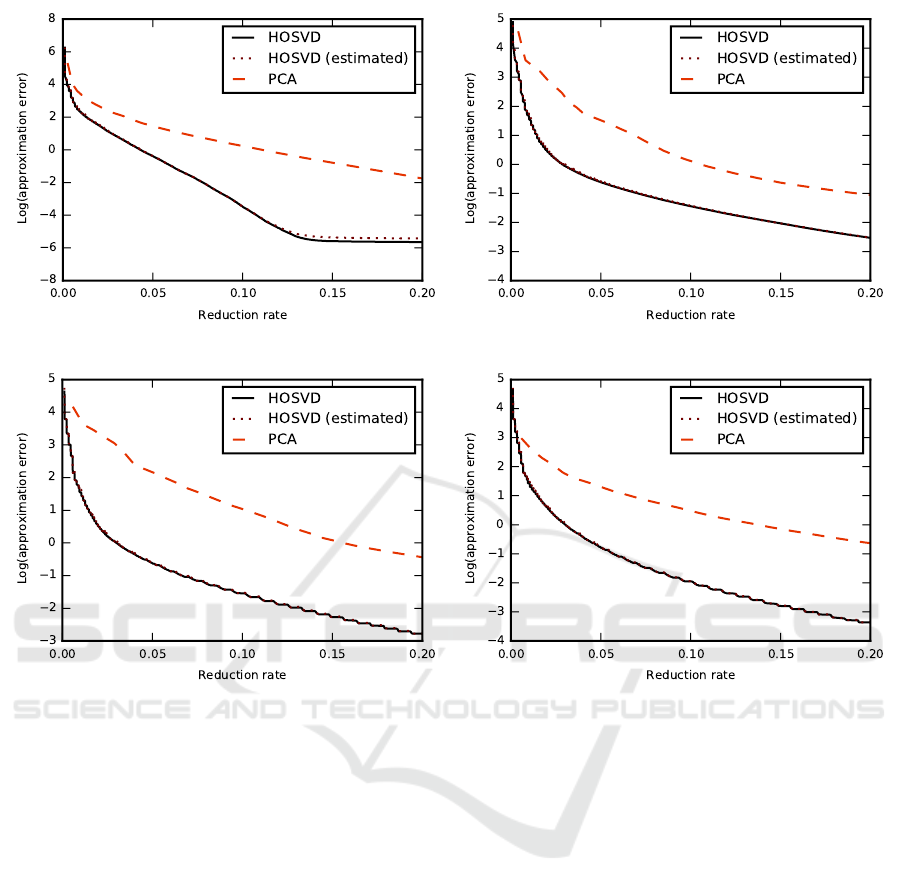
(a) (b)
(c) (d)
Figure 1: Rate-distortion curves for animations: chicken (a), march (b), crane (c), samba (d). The horisontal axis represents
the reduction rate Θ(
˜
T
ik
) and the vertical axis is the logarithm of reconstruction error e
kg
(T ,
˜
T ). Plots present actual and
estimated error values for HOSVD. Error values for PCA are provided for reference. The difference between the estimated
and actual values of approximation error for HOSVD are very small.
3.2 Results
The reconstruction error introduced by HOSVD ap-
proximation of TCMS data is presented in Fig. 3.
Each pixel in panels (a), (c) and (e) represents the N-
rank reconstruction while axes show the number of
mode-1 and mode-3 components. The error is mono-
tonic and it drops sharply from the highest value in the
lower-left corner (reconstruction from only one com-
ponent in both modes) to the low error value in the
upper-right corner. The perceptual distortion of re-
constructed animation becomes very small for ∼ 50
mode-1 and mode-3 components which corresponds
to values lying above and on the right from the isoline
zero.
Panels (b), (d) and (f) in Fig. 3 represent the corre-
sponding values of the estimation error ψ(T ,
˜
T
ik
). We
can imminently see that ψ(T ,
˜
T
ik
) values are small.
That means that the error estimation obtained using
Eq. (12) is close to its actual value. However, it is
apparent that the estimation is more accurate for large
error values in the upper-left and lower-right corners,
separated with the isoline (−8). At the same time
an obvious strategy for optimal N-rank choice are the
values close to the diagonal line connecting the lower-
left and upper-right corners of the array. These param-
eters results in low reconstruction error but are also
less accurately estimated. Nevertheless, for parame-
ters representing the perceptually acceptable TCMS
approximation, the estimation is accurate enough that
there is no difference in the parameter choice based
on estimated or accurate error values.
The rate-distortion curves for actual and estimated
values of HOSVD approximation error are presented
in Fig. 1. PCA approximation error is provided for
reference. The perceptual distortion of the animation
VISAPP 2016 - International Conference on Computer Vision Theory and Applications
144
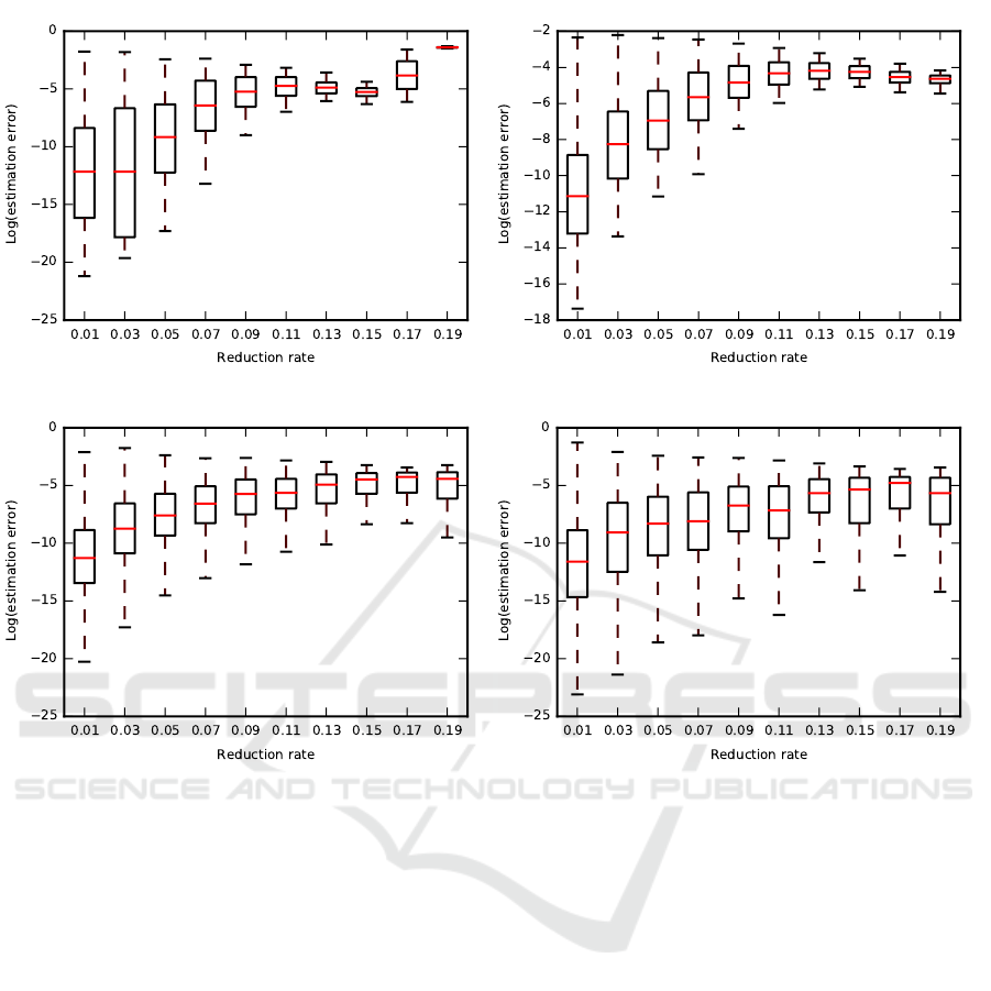
(a) (b)
(c) (d)
Figure 2: Estimation error for animations: chicken (a), march (b), crane (c), samba (d). The horisontal axis represents the
reduction rate Θ(
˜
T
ik
) and the vertical axis is the logarithm of estimation error ψ(T ,
˜
T
ik
). Each error bar represents the median,
lower and upper quantile as well as error range in one of ten non-overlaping windows of equal length. Values on the horizontal
axis are in the middle of a corresponding window.
becomes acceptable for reduction rate ∼ 5% original
data size, and almost indistinguishable when the re-
duction rate is ∼ 10% of the original size.
Fig. 2 is the visualization of estimation error for
our animations. Each error bar represents the median,
lower and upper quantile and error range in the ten
non-overlaping horizontal windows. As we can see
the estimation is more precise for high reduction rate,
but with significant variance. This is more visible
for artificial chicken sequence than for motion-capture
animations. This effect results mostly from the im-
proper estimation for very low N-rank values located
in the lower-left corner of the parameter array. On the
other hand, for lower reduction rate the estimator is
less precise but with a low variance.
4 CONCLUSIONS
We have shown how to estimate the N-rank HOSVD
reconstruction error for TCMS data. We argue that for
representative sequences the estimator is saturated.
That means that the estimated distortion is very close
to its actual value and can aid in selection of approx-
imation parameters. Expressing the distortion result-
ing from approximation of T in the form of KG error
is useful during the creation of HOSVD-based TCMS
compression algorithms.
ACKNOWLEDGEMENTS
This work has been partially supported by the
project ‘Representation of dynamic 3D scenes
Parameter Estimation for HOSVD-based Approximation of Temporally Coherent Mesh Sequences
145
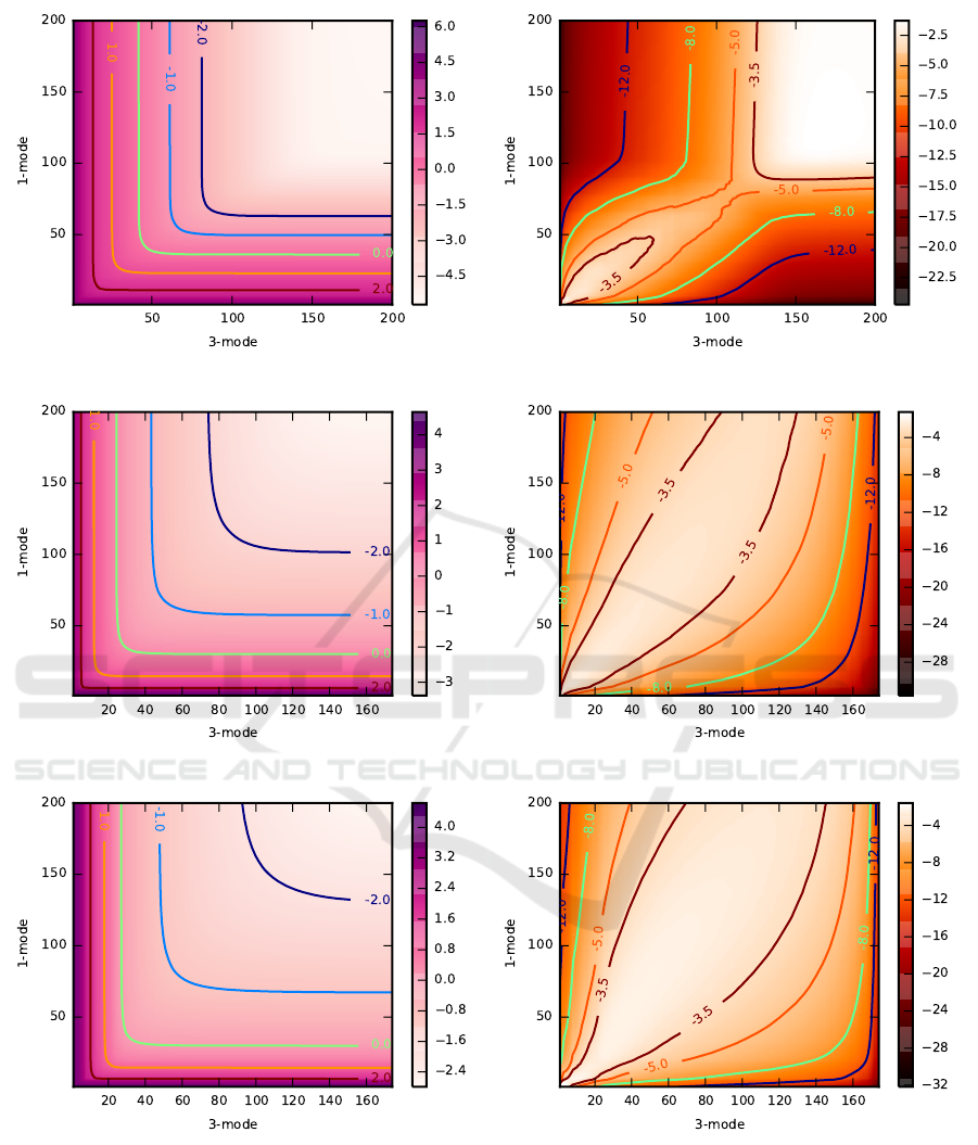
(a) (b)
(c) (d)
(e) (f)
Figure 3: Reconstruction and estimation errors for three animations: chicken (the upper row), crane (the middle row), samba
(the lower row). Pixels in arrays (a),(c) and (e) represent the logarithm of e
kg
(T ,
˜
T
ik
) as a function of the number of mode-1
and mode-3 components used for reconstruction. Arrays (b),(d) and (f) present the corresponding estimation errors ψ(T ,
˜
T
ik
)
defined by Eq. (13).
using the Atomic Shapes Network model’ fi-
nanced by National Science Centre, decision DEC-
2011/03/D/ST6/03753. We would like to thank our
reviewers for their insightful comments. We would
also like to thank P. Gawron for fruitful discussions.
VISAPP 2016 - International Conference on Computer Vision Theory and Applications
146

REFERENCES
Alexa, M. and Muller, W. (2000). Representing animations
by principal components. In Computer Graphics Fo-
rum, volume 19, pages 411–418. Citeseer.
Arcila, R., Cagniart, C., H
´
etroy, F., Boyer, E., and Dupont,
F. (2013). Segmentation of temporal mesh sequences
into rigidly moving components. Graphical Models,
75(1):10–22.
Ballester-Ripoll, R. and Pajarola, R. (2015). Lossy volume
compression using tucker truncation and thresholding.
The Visual Computer, pages 1–14.
De Lathauwer, L., De Moor, B., and Vandewalle, J.
(2000). A multilinear singular value decomposition.
SIAM journal on Matrix Analysis and Applications,
21(4):1253–1278.
Jolliffe, I. (2005). Principal component analysis. Wiley
Online Library.
Karni, Z. and Gotsman, C. (2004). Compression of soft-
body animation sequences. Computers & Graphics,
28(1):25–34.
Kolda, T. G. and Bader, B. W. (2009). Tensor Decomposi-
tions and Applications. SIAM Review, 51(3):455–500.
Maglo, A., Lavou
´
e, G., Dupont, F., and Hudelot, C. (2015).
3d mesh compression: Survey, comparisons, and
emerging trends. ACM Computing Surveys (CSUR),
47(3):44.
Romaszewski, M., Gawron, P., and Opozda, S. (2013). Di-
mensionality reduction of dynamic mesh animations
using ho-svd. Journal of Artificial Intelligence and
Soft Computing Research, 3(4):277–289.
V
´
a
ˇ
sa, L. and Skala, V. (2009). Cobra: Compression of the
basis for pca represented animations. In Computer
Graphics Forum, volume 28, pages 1529–1540. Wi-
ley Online Library.
Parameter Estimation for HOSVD-based Approximation of Temporally Coherent Mesh Sequences
147
