
VAR a New Metric of Cryo-electron Tomography Resolution
Hmida Rojbani
1,2
and Atef Hamouda
2
1
University of Strasbourg, 67412, Illkirch Cedex, France
2
Faculty of Science of Tunis, University Tunis El Manar, 2092 El Manar Tunis, Tunisia
Keywords:
Electron Tomography, Resolution, Metric, 3D Structures, Tilt Angles.
Abstract:
Motivate by reaching a better understanding of the biological cells, scientists use the Transmission Electron
Microscope (TEM) to investigate their inner structures. The cryo-electron tomography (cryo-ET) offers the
possibility to reconstruct 3D structure reconstruction of a cell slice, that by tilting it according different an-
gles. The resolution limits is the biggest challenge in the cryo-ET. The two phases involved in increasing the
resolution are the acquisition phase and the reconstruction phase. In this work, we focus in the last one, as the
biologists treat the acquisition phase within the phase of acquisition itself. The resolution of reconstruction
depends on many factors such as: (1) the noisy and missing information from the collected projections data,
(2) the capacity of processing large data sets, (3) the parametrization of the contrast function of the micro-
scope, (4) errors of the tilt angles used in projections. In this paper, we presented a new method to evaluate
the resolution of a reconstruction algorithm. Then the proposed method is used to show the relation between
errors of the tilt angles used in projection and the degradation of the resolution. The resolution evaluation tests
are made with different reconstruction methods (analytic and algebraic) applied on synthetic and real data.
1 INTRODUCTION
The resolution is a key characteristic of the 3D re-
constructed object, it affects the visual quality of the
object and it can limit the performance of the segmen-
tation method if it fails to attain the highest level pos-
sible. The highest reachable resolution in cryo-ET is
around 5
˚
A, which allows us to locate small objects
as ribosomes, nucleosomes, .... As requirement to
achieve such resolution one must lower the dose of
electrons used on the specimen during the acquisition
and that to minimize the weight of radiation damage
(Egerton et al., 2004). This reduction decreases the
signal to noise ratio and delivers low contrast image.
Moreover, the thickness of the ice used in the fixation
of the sample affects also the final resolution of the
reconstructed volume (Stagg et al., 2006). Therefore,
the techniques requested to obtain high-resolution 3D
structures must be refined in order to handle the low
contrast and at the same time very noisy data (Sorzano
et al., 2004).
Mainly, the reconstruction methods that are used
in cryo-ET, they are belongs to two different fam-
ily: (i) the analytic family, where we find meth-
ods as filtered back-projection methods, or direct
Fourier inversion methods implemented in Fourier
space (Penczek, 2010); (ii) the algebraic family,
where iterative real-space methods are implemented,
such as ART (Gordon et al., 1970) or SIRT (Gilbert,
1972).
In fact, we will focus in this paper on the resolu-
tion, specifically how we can judge if this resolution
is a high resolution or not? The rest of the paper will
be structured as follows: in section 2, we discuss the
resolution in the literature, and we present the differ-
ent method of reconstruction found in the literature
in section 3. In section 4, we give our approach for
judging the resolution quality; followed by present-
ing the evaluation of the results in section 5. Finally,
we summarize and give some perspectives.
2 RESOLUTION: DEFINITION
AND METHODS
One of the conversional question in the image-
processing field is how we can define the resolution of
an image. The term ”resolution” in its popular knowl-
edge refers to the pixel count or the dimensions of an
image. Unfortunately,this opinion has no real relation
with the true meaning of the term resolution. Resolu-
tion is simply the ability to tell if a set of pixels rep-
resents distinct object rather than one object (cf. red
156
Rojbani, H. and Hamouda, A.
VAR a New Metric of Cryo-electron Tomography Resolution.
DOI: 10.5220/0005725801540159
In Proceedings of the 11th Joint Conference on Computer Vision, Imaging and Computer Graphics Theory and Applications (VISIGRAPP 2016) - Volume 3: VISAPP, pages 156-161
ISBN: 978-989-758-175-5
Copyright
c
2016 by SCITEPRESS – Science and Technology Publications, Lda. All rights reserved
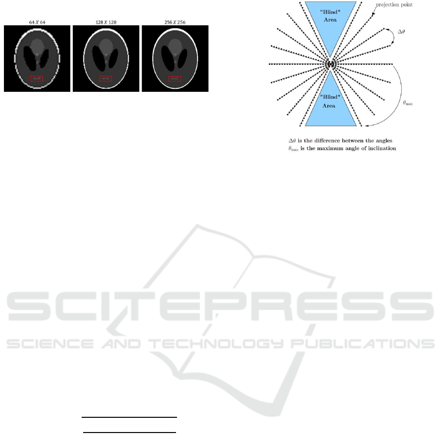
rectangles in Fig. 1).
Figure 1: Effect of pixel resolution.
In electron microscopy, our field of interest, res-
olution (A.K.A spatial resolution) refers to the mini-
mum distance between adjacent and in the same time
distinguishable objects in the image; which can be
both detected and interpreted (O’Keefe and Allard,
2004).
Another definition of spatial resolution is given by
(Midgley and Weyland, 2003), where if the alignment
condition of the projection images is satisfied, the res-
olution of the reconstructed object will be depends
from number of projection used in the reconstruction
(n
θ
), maximum angle reached in the tilting operation
(θ
max
) (cf. Fig. 2) and the lateral dimension of the re-
constructed volume (D). The resolution is different
in each axis of the plan. Let us assume that that the
object is in OXYZ space, the axis of tilt is parallel to
the axis OX and the electron beam is parallel to the
OZ axis. Thus, it is possible to define the spatial res-
olution of the reconstructed volume along three plans
as:
• XY: the resolution is equal to the resolution of the
original 2D projections.
• XZ: the resolution is defined as πD/n
θ
.
• ZY: the resolution is degraded by a factor e
yz
from
the resolution of XZ. This factor is equal to :
e
yz
=
s
θ
max
+ sinθ
max
cosθ
max
θ
max
− sinθ
max
cosθ
max
We have another idea to determine the spatial res-
olution; our idea is based on a simulation of our vi-
sual experience with the image. The aim of proposing
this new approach is to verify the truth of argument
that said the uncertainty on the tilt angles due to me-
chanical imprecision of the TEM has no effect on the
final reconstructed object resolution (Colliex, 1998).
To test this theory, we used different reconstruction
method that are presented in the next section.
Figure 2: Illustration of sampling data in the Fourier space.
3 RECONSTRUCTION METHODS
In this section, we will discuss the commonly used
methods in cryo-ET reconstruction. In general, there
are two major families of tomographic reconstruction
methods (Frank, 2006). One is the set of analytical
algorithms, based on the direct data inversion. The
other is the set of algebraic (iterative) methods, based
on the inverseproblem, which seeks to reconstruct the
object by iteratively optimizing a criterion defining a
range fidelity between the real projections data and
the reconstructed object.
Analytical methods can use the fast Fourier trans-
form in the calculation of the solution, which can
accelerate the execution time of tomographic recon-
struction. This is a considerable advantage com-
pared to iterative methods. However, an analytical
reconstruction will be effective only if the number of
projection is high and they are uniformly distributed
around the object, which is not the case of cryo-ET.
Moreover, analytical methods are not adapted to the
introduction of additional information on the object
to be used in reconstruction to increase its effective-
ness. For this reason, we will concentrate only on the
algebraic reconstruction.
As mentioned above many algebraic reconstruc-
tions algorithm exist in the literature. In this paper,
we will concentrate in how the model of pixels dis-
tribution in the projection are calculated, not in how
the reconstruction algorithm works. In general, the
problem of tomography represented by the relation
between the projections p
θ
i
provided by the micro-
scope according to angle θ
i
and the reconstructed ob-
ject f, as follows:
p
θ
i
= W
θ
i
f, (1)
Thereby, the projection problem is modeled as an
VAR a New Metric of Cryo-electron Tomography Resolution
157
equation system whose matrix W
θ
i
is sparse. The ma-
trix W
θ
i
holds the coefficients of the projections ac-
cording to the angle θ
i
; ∀i ∈ [1 n
θ
]. Here, our target is
which is the best method to find W
θ
i
or which method
provide better resolution with a small number of pro-
jection (n
θ
).
3.1 Modelisation of the Projection
Matrix W
θ
i
A reconstruction of good quality requires accurate
modelling of the data acquisition process, or the pro-
jection matrix. Several methods are proposed in the
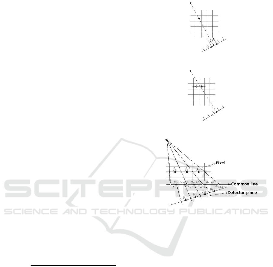
literature to model this matrix. Standard models such
as ”voxel driven” and ”ray driven” (Joseph, 1982) are
based on direct sampling, which gives modelling er-
rors and artifacts in the reconstructed image. The
model ”voxel driven” (cf. Fig. 3(a)) is based on con-
necting the source to the projection plane by passing a
line through the middle of voxel of interest. However,
the model ”ray driven” (cf. Fig. 3(b)) is based on con-
necting the source to the centre of the cell of interest
on the projection plan by a passing a line through the
image.
To overcome the shortcoming of these two algo-
rithm, (Man and Basu, 2004) proposed another model
called ”distance driven” that modelled the line projec-
tion in the shape of stairs to give a better modelling.
This method’s role is to match the borders of each
voxel and the borders of each cell of the projection
plan on a common line; the difference between these
points defines the projection coefficients. Measure the
exact intersection area is a difficult task, for this rea-
son, this area will be approximated. For example, to
estimate the projection coefficient p
2
in Fig. 3(c), we
can use the follow equation (Chen et al., 2015):
∆
p
2
=
(x
n+1
− y
m+1
) f
1
+ (y
m+2
− x
n+1
) f
2
y
m+2
− y
m+1
This is the usual method used in the cryo-ET algebraic
reconstruction.
Recently, Momey et al. (Momey et al., 2011) pro-
posed the use of B-splines as an alternative to the ap-
proach of ”distance driven” (cf. Fig. 3(c)). The B-
Splines are piecewise polynomials, which are charac-
terized by the degree of the constituent polynomials.
The recent work of the sampling theory, (Thevenaz
et al., 2000) (Unser, 2000), have demonstrated their
effectiveness to represent a continuous signal with
good accuracy. One of the most significant enhance-
ments provided by the new approach ”spline driven”
proposed by Momey et al. (Momey et al., 2014) is the
reduction of the angular sampling projections with-
out any quality loss. Indeed, this method is based on
(a) ”voxel driven” (Man and Basu, 2004)
(b) ”ray driven” (Man and Basu, 2004)
(c) ”distance driven” (Chen et al., 2015)
Figure 3: The various methods to create a projection matrix.
the idea of presenting the objects in the image by B-
splines instead of using classical cubic grid. Even the
lines of projections are modelled by B-splines. This
model improves the calculation of the projection co-
efficients.
In this paper, we want to verify if the using of the
iterative algebraic methods can affect and decrease
the resolution of the reconstruction or not. For this,
we will compare between SIRT (with the ”distance
driven”) and the filtered back-projection (FBP), us-
ing our new metric of resolution. More details of
this approach called Visual Assumption of Resolution
(VAR) is in the next section.
4 VISUAL ASSUMPTION OF
RESOLUTION
The aim of using electron microscopy is reaching an
atomic resolution, which is a hard target to reach in
VISAPP 2016 - International Conference on Computer Vision Theory and Applications
158

the biological imaging case, due to the sensibility na-
ture of biological simples to electron radiation. The
solution was to minimize in one side the electron dose
used in acquisition (providing a low contrast image
with low SNR) and in the other side the number of ex-
posing to this dose (providing a small number of pro-
jection leading to a mediocre reconstruction). In this
work, we will concentrate only on the effect of the
projections number putting in mind that in the syn-
thetic tests we will control everything else to be in the
perfect conditions. The purpose of our metric VAR is
to see how much is the loss of resolution according to
the real objects resolution.
If we analyze visually the reconstructed object we
find that the building shape of objects in the image
change dramatically according to number of iteration
of the reconstruction algorithm, the number of pro-
jection (n
θ
) used in reconstruction (cf. Fig. 4). The
changes can be described by perturbation in the bor-
ders of object, which leads to fusion of object if they
are near each other. In addition, there are a slight
change in the spectral of the object. Hence, we have
the idea of using these two modification to calculate
the rate of loss in resolution from the real object.
Figure 4: Resolution decrease after reconstruction with
SIRT (100 iteration) and n
θ
= 71.
The VAR metric has two section, the first interpret
the space (pixel) diversity between the original and re-
constructed image (noted as VAR
space
) and the second
outline their the spectral (radiometry) variation (noted
as VAR
spectral
).
To calculate VAR
space
we will count the differ-
ence between the nonzero number of pixel in the orig-
inal image and in the reconstructed image. The found
value will be normalized by the nonzero number of
pixel in the original image. The equation to calculate
VAR
space
as follow:
VAR
space
=
|
∑
N
i=1
R
i
−
∑
N
i=1
O
i
|
∑
N
i=1
O
i
(2)
Where N is the total number of pixel in the image,
R
i
= 1 (respectively O
i
= 1) if the i−th pixel of the re-
constructed (respectively original) image is nonzero,
R
i
= 0 (respectively O
i
= 0) otherwise. VAR
space
will
equal to zero if two image has the same number of
nonzero pixels, otherwise will be greater than zero.
Now, to calculate VAR
spectral
we will count the
difference between the sum of the spectral of all pix-
els between the original image and the reconstructed
image. As the previous calculation, the difference will
be normalized by the sum of the original image. The
equation to calculate VAR
space
as follow:
VAR
spectral
=
|
∑
N
i=1
PxR
i
−
∑
N
i=1
PxO
i
|
∑
N
i=1
PxO
i
(3)
Where PxR
i
(respectively PxO
i
) is the spectral of
the i− th pixel of the reconstructed (respectively origi-
nal). The same as the previous, VAR
spectral
will equal
to zero if two image has the same amount of radiome-
tries, otherwise will be greater than zero.
The value of VAR will be the mean between
VAR
space
and VAR
spectral
.
VAR =
VAR
space
+VAR
spectral
2
(4)
One can notice that for VAR to be efficient the
tested image must simple structured. The tests and
results of applying VAR in different situations are
shown in the next section.
5 RESULTS
Several experiments were conducted to assess the
efficiency of the proposed method on 2D and 3D
data. The experiments involve 62 2D and 25 3D syn-
thetic gray-level images randomly generated at dif-
ferent size N = 128, 256, 512. A sample of 2D the
synthetic images used are shown in the figure 5.
Figure 5: 2D synthetic images.
We will calculate also the cross-correlation coef-
ficient (equation (5)). It is a criterion to measure the
degree of similarity between the original image and
the reconstructed image. This coefficient is equal to 1
when the reconstructed image coincides exactly with
the original image and zero otherwise.
Corr =
∑
N
i=1
(PxO
i
− M(O))(PxR
i
− M(R))
q
∑
N
i=1
(PxO
i
− M(O))
2
∑
N
k=1
(PxR
i
− M(R))
2
(5)
where M(.) is the mean of the radiometry of the
image.
VAR a New Metric of Cryo-electron Tomography Resolution
159

The first phase of testing was to study the effect of
different number projection (n
θ
) over the resolution
of the reconstruction. For the record, all the algebraic
reconstruction in this section used a fixed number of
iteration equals to 100 iterations. The mean results
are shown in table 1 and table 2.
Table 1: The mean evaluation of 2D and 3D synthetic data
for the FBP.
Size 128 256 512
Corr 0.89 0.93 0.95
VAR 0.67 0.59 0.58
Table 2: The mean evaluation of 2D and 3D synthetic data
for the SIRT with ”distance driven” method.
Size 128 256 512
Corr 0.92 0.95 0.96
VAR 0.52 0.39 0.31
We can see clearly the upper hand of the SIRT
over the FBP. Moreover, we notice in table 1 that even
if the correlation is good, the resolution was poor. For
this reason, we can say that correlation is not a trusted
evaluation measure to prove the performance of a re-
construction. In the followed tests, we calculate only
VAR.
The mean results according to deferent angular er-
ror (AE) applied on tilt angles are given in table 3 for
n
θ
= 360 and in table 4 for n
θ
= 71, which is the usual
number used in the real case of cryo-ET.
Table 3: The results for 3D synthetic data with n
θ
= 360.
AE
0
◦
≤ 1
◦
≤ 2
◦
FBP 0.56 0.88 0.92
SIRT 0.15 0.23 0.34
Table 4: The results for 3D synthetic data with n
θ
= 71.
AE
0
◦
≤ 1
◦
≤ 2
◦
FBP 0.82 0.99 1.32
SIRT 0.24 0.38 0.57
It is clear that if the tilt angles are erroneous, than
the resolution will decrease even if we use all the pos-
sible tilt angles.
6 CONCLUSION
In this paper, we proposed a new metric to calculate
the resolution of the reconstruction object. The pur-
pose of this metric VAR is to verify to performance
of the reconstruction algorithm used and their effi-
ciency to preserve the resolution of the real object.
We showed here, the upper hand of the algebraic iter-
ative methods. In addition, we showed also the effect
of an erroneous tilt angles over the results of the re-
constructed object.
REFERENCES
Chen, J.-L., Li, L., Wang, L.-Y., Cai, A.-L., Xi, X.-Q.,
Zhang, H.-M., Li, J.-X., and Yan, B. (2015). Fast par-
allel algorithm for three-dimensional distance-driven
model in iterative computed tomography reconstruc-
tion. Chinese Physics B, 24(2).
Colliex, C. (1998). The Electron Microscopy. Presses Uni-
versitaires de France.
Egerton, R., Li, P., and Malac, M. (2004). Radiation dam-
age in the TEM and SEM. Micron, 35(6):399–409.
Frank, J. (2006). Electron tomography: methods for three-
dimensional visualization of structures in the cell.
Springer.
Gilbert, P. (1972). Iterative methods for the three-
dimensional reconstruction of an object from projec-
tions. Journal of Theoretical Biology, 36(1):105–117.
Gordon, R., Bender, R., and Herman, G. (1970). Al-
gebraic Reconstruction Techniques (ART) for three-
dimensional electron microscopy and X-ray photog-
raphy. J Theor Biol, 29(3):471–481.
Joseph, P. (1982). An improved algorithm for reprojecting
rays through pixel images. Medical Imaging, IEEE
Transactions on, 1(3):192–196.
Man, B. D. and Basu, S. (2004). Distance-driven projection
and backprojection in three dimensions. Physics in
Medicine and Biology, 49(11):2463.
Midgley, P. and Weyland, M. (2003). 3d electron mi-
croscopy in the physical sciences: the development
of z-contrast and {EFTEM} tomography. Ultrami-
croscopy, 96(34):413 – 431. Proceedings of the In-
ternational Workshop on Strategies and Advances in
Atomic Level Spectroscopy and Analysis.
Momey, F., Denis, L., Mennessier, C., Thiebaut, E., Becker,
J.-M., and Desbat, L. (2011). A new representation
and projection model for tomography, based on sep-
arable b-splines. In Nuclear Science Symposium and
Medical Imaging Conference (NSS/MIC), 2011 IEEE,
pages 2602–2609.
Momey, F., Thiebaut, E., Mennessier, C., Denis, L., and
Becker, J.-M. (2014). Spline driven: high accuracy
projectors for 3D tomographic reconstruction from
few projections. submitted.
O’Keefe, M. and Allard, L. (2004). A standard for
sub-ngstrom metrology of resolution in aberration-
corrected transmission electron microscopes. Mi-
croscopy and Microanalysis, 10:1002–1003.
Penczek, P. (2010). Chapter one - fundamentals of
three-dimensional reconstruction from projections. In
Grant, J., editor, Cryo-EM, Part B: 3-D Reconstruc-
tion, volume 482 of Methods in Enzymology, pages
1–33. Academic Press.
VISAPP 2016 - International Conference on Computer Vision Theory and Applications
160

Sorzano, C., de la Fraga, L., Clackdoyle, R., and Carazo, J.
(2004). Normalizing projection images: a study of im-
age normalizing procedures for single particle three-
dimensional electron microscopy. Ultramicroscopy,
101(24):129–138.
Stagg, S., Lander, G., Pulokas, J., Fellmann, D., Cheng, A.,
Quispe, J., Mallick, S., Avila, R., Carragher, B., and
C.S.Potter (2006). Automated cryo-em data acquisi-
tion and analysis of 284742 particles of groel. J Struct
Biol, 155:470–481.
Thevenaz, P., Blu, T., and Unser, M. (2000). Interpolation
revisited [medical images application]. Medical Imag-
ing, IEEE Transactions on, 19(7):739–758.
Unser, M. (2000). Sampling-50 years after shannon. Pro-
ceedings of the IEEE, 88(4):569–587.
VAR a New Metric of Cryo-electron Tomography Resolution
161
