Towards Energy-efficient Collision-free Data Aggregation Scheduling in
Wireless Sensor Networks with Multiple Sinks
Sain Saginbekov
1,3
, Arshad Jhumka
2
and Chingiz Shakenov
3
1
Department of Computer Science, Nazarbayev University, Astana, Kazakhstan
2
Department of Computer Science, University of Warwick, Coventry, CV4 7AL, U.K.
3
Department of Computer Science, National Laboratory Astana, Astana, Kazakhstan
Keywords:
Wireless Sensor Networks, Data Aggregation Scheduling, Multiple Sinks, Many-to-many Communication,
Routing, MAC.
Abstract:
Traditionally, Wireless Sensor Networks (WSNs) are deployed with a single sink. Due to the emergence of
sophisticated applications, WSNs may require more than one sink, where many nodes forward data to many
sinks. Moreover, deploying more than one sink may prolong the network lifetime and address fault tolerance
issues. Several protocols have been proposed for WSNs with multiple sinks. However, they are either routing
protocols or forward data from many nodes to one sink. In this paper, we propose data aggregation scheduling
and energy-balancing algorithms for WSNs with multiple sinks that forward data from many nodes to many
sinks. The algorithm first forms trees rooted at virtual sinks and then balances the number of children among
nodes to balance energy consumption. Further, the algorithm assigns contiguous slots to sibling nodes to
avoid unnecessary energy waste due to active-sleep transitions. We prove a number of theoretical results and
the correctness of the algorithms. Simulation and testbed results show the correctness and performance of our
algorithms.
1 INTRODUCTION
A wireless sensor network (WSN) consists of a set of
resource-constrained devices, called nodes, that com-
municate wirelessly via radio. These nodes sense the
environment for events of interest and subsequently
relay the information to a dedicated device called a
sink, with data from several nodes aggregated along
the way for energy efficiency reasons. The data can
then later be analysed offline.
Traditionally, WSNs have been deployed with a
single sink (Akyildiz et al., 2002). However, there are
several reasons that limit the usefulness of a single
sink. For example, the emergence of more sophisti-
cated applications require more than one sink (Mot-
tola and Picco, 2011). Moreover, deploying more
than one sink may improve network throughput and
prolong network lifetime by balancing energy con-
sumption, and may address fault tolerance issues (Lee
et al., 2005; Valero et al., 2012; Sitanayah et al., ).
In WSNs, TDMA-based protocols are often used
to avoid message collisions and guarantee timeliness
properties. Also, TDMA-based protocols have the ad-
vantages of avoiding idle listening and overhearing.
TDMA MAC protocols work by breaking the time-
line into slots and assigning those slots to nodes. Each
node then can only transmit in a slot it has been as-
signed. Lots of TDMA-based protocols have been
proposed (Rajendran et al., 2005; Rajendran et al.,
2006; Sohrabi et al., 2000). However, most TDMA-
based MAC protocols have been developed with a sin-
gle sink assumption. In a WSN with multiple sinks,
such slot assignment will result in a very high latency
for one of the sink.
Thus, this implies that there is a need for TDMA-
based MAC protocols specifically for WSNs with
multiple sinks. There is a dearth of work in this area.
Data aggregation scheduling (DAS) algorithms
in a WSN with multiple sinks have been presented
in (Kawano and Miyazaki, 2008; Bo and Li, 2011).
However, in the works, the data aggregation schedul-
ing is done from many nodes to one sink, whereas this
paper considers the data aggregation scheduling from
many nodes to many sinks.
One way to solve the data aggregation scheduling
problem in WSNs with multiple sinks is to first de-
velop a backbone that connects sinks and then allocate
slots to nodes that connect to the backbone. The prob-
Saginbekov, S., Jhumka, A. and Shakenov, C.
Towards Energy-efficient Collision-free Data Aggregation Scheduling in Wireless Sensor Networks with Multiple Sinks.
DOI: 10.5220/0005735000770086
In Proceedings of the 5th International Confererence on Sensor Networks (SENSORNETS 2016), pages 77-86
ISBN: 978-989-758-169-4
Copyright
c
 2016 by SCITEPRESS – Science and Technology Publications, Lda. All rights reserved
77

lem of developing the backbone, i.e., connecting the
sinks is directly related to the problem of developing
a Steiner tree (Gilbert and Pollak, 1968). In this case,
we are interested in developing a minimum Steiner
tree, which is known to be NP-complete (Karp, 1972).
To address the computational complexity of this prob-
lem, there are different ways of going about it. One
of them is to look at specific instances of the prob-
lem that can lead to a polynomial-time solution to the
problem. In this paper, we focus on the problem with
2 sinks, since the minimum Steiner tree can be com-
puted in polynomial-time, as the minimum Steiner
tree is the shortest path between the sinks. How-
ever, our proposed algorithm for 2 sinks also works
for WSNs with more than 2 sinks, but in sub-optimal
ways.
In this context, we make the following novel con-
tributions:
• We formalise the problem of DAS scheduling in a
WSN.
• We prove a number of impossibility results, as
well as show a lower bound for solving a variant
of DAS called weak DAS.
• We propose two algorithms, which taken together,
solves weak DAS and results in a schedule that
matches the predicted lower bound.
• Through experiments, we show the performance
and correctness of the algorithms.
The rest of the paper is organized as follows. In
Section 2, we present an overview of related work.
In Section 3, we formalise the problem of Data Ag-
gregation Scheduling (DAS) in a WSN. Then, in Sec-
tion 4, we prove a number of impossibility results,
as well as show a lower bound for solving a vari-
ant of DAS called weak DAS. Further, in Section 5,
we propose two algorithms, called Balancing Tree
Formation (BTF) and Energy-Efficient Collision Free
(EECF), which taken together, solves weak DAS and
results in a schedule that matches the predicted lower
bound. In Section 6, we present experimental setup.
Finally, in Section 7, through simulations, we show
the correctness and performance of our algorithms.
2 RELATED WORK
Protocols that have been developed on communica-
tion for WSNs with multiple sinks can be found
in(Mottola and Picco, 2011; Kawano and Miyazaki,
2008; Bo and Li, 2011; Thulasiraman et al., 2007;
Tuysuz Erman and Havinga, 2010; Hui Zhou and Xu,
2012). A scheme proposed in (Mottola and Picco,
2011) performs data collection from many nodes to
many sinks. The main idea of the protocol is to de-
crease the number of redundant transmission by us-
ing information about the neighbours. In (Thulasir-
aman et al., 2007), authors propose an algorithm that
builds two node-disjoint paths from every node to two
different (drains) sinks. If one of two paths fails,
the other is used to route the data. In (Tuysuz Er-
man and Havinga, 2010), authors propose a routing
protocol that is based on hexagon-based architecture.
Nodes in the network is grouped into hexagons ac-
cording to their locations. A routing protocol pro-
posed in (Hui Zhou and Xu, 2012), is based on trees.
In the protocol, different trees rooted at different
sinks are used to forward data. These algorithms ad-
dress the problem at routing level, i.e., none of these
schemes provide a MAC layer protocol.
The work presented in (Kawano and Miyazaki,
2008; Bo and Li, 2011) have more relevance to our
work. In (Kawano and Miyazaki, 2008), in addition
to an algorithm that forms shortest path trees rooted at
each sink in a WSN with multiple sinks, authors pro-
pose a scheduling algorithm that use a graph colour-
ing algorithm. So, nodes send to their nearest sink
without collision. The authors of (Bo and Li, 2011),
propose two algorithms for scheduling data aggrega-
tion in multiple-sink sensor networks. The first of
the algorithm is Voronoi-based scheduling where the
sensing area is divided into regions forming k forests,
one forest for each sink. Then the algorithm makes
schedules for nodes. The second algorithm is Inde-
pendent scheduling which differs from the first al-
gorithm in forest construction. However, in both of
the algorithms different portions of sensor nodes send
their data to a single different sink, i.e., many-to-one
communication, whereas we consider the case where
many nodes send their data to many sinks (many-to-
many).
3 PROBLEM FORMULATION
We present the following definitions that we will use
in this paper.
Definition 1 (Schedule). A schedule S : V → 2
N
is a
function that maps a node to a set of time slots.
Definition 2 (DAS-label). Given a network G =
(V, E), a sink ∆, a schedule S and a path γ = n ·
m.. . ∆, we say that n is DAS-labeled under S on γ
for ∆ if ∃t ∈ S (n) · ∃t
0
∈ S (m) : t
0
> t.
We call the node m on γ the ∆-parent of n and γ
the DAS-path for n.
Definition 3 (Strong and Weak Schedule). Given a
network G = (V, E), a sink ∆ ∈ V and a schedule S,
SENSORNETS 2016 - 5th International Conference on Sensor Networks
78

S is said to be a strong DAS schedule for ∆ for a node
n ∈V iff ∀ path γ
i
= n·m
i
. . . ∆, n is DAS-labeled under
S on γ
i
for ∆. S is a weak DAS schedule for ∆ for n if
∃ path γ = n ·m
i
. . . ∆ such that n is DAS-labeled under
S on γ for ∆.
A schedule S is strong DAS (resp. weak DAS) for
G iff ∀n ∈ V , S is strong DAS schedule (resp. weak
DAS schedule) for ∆ for n.
We will only say a strong or weak schedule when-
ever ∆ is obvious from the context. A strong sched-
ule, in essence, is resilient to problems that occur in
the network such as radio links not working or node
crashes during deployment. On the other hand, a
weak schedule is not resilient and, any problem hap-
pening, will entail that a message from node n to m
will be lost.
It has been shown in (Jhumka, 2010) that it is im-
possible to develop strong schedules.
Given a network with 2 sinks ∆
1
, ∆
2
, we wish to
develop a weak schedule for ∆
1
and ∆
2
. There are sev-
eral possibilities to achieve this. In general, to develop
a weak schedule, several works have adopted the ap-
proach whereby a tree is first constructed, rooted at
the sink, and then slots assigned along the branches to
satisfy the data aggregation constraints. A trivial so-
lution is to construct two trees, each rooted at a sink,
and then to assign slots to nodes along the trees. This
means that nodes can have two slots, i.e., meaning
that nodes may have to do two transmissions for the
same message. Thus, we seek to reduce the number
of slots for nodes to transmit in.
3.1 DAS Scheduling
We model our problem as follows:
We capture slots assignment with a set of decision
variables.
t
S
n
=

1 t ∈ S(n)
0 otherwise
A set value assignment to these variables represent a
possible schedule. The number of slots used, which
equates to the number of transmission by nodes, has
to be reduced for extending the lifetime of the net-
work. The number of slots used is given by:
numSlots
S
=
∑
t∈T,n∈V
t
S
n
(1)
We also capture the number of nodes with multiple
slots as follows:
f
S
n
=

1 |S(n)| > 1
0 otherwise
However, such a schedule may not assign a slot to a
given node, so we need to rule out some schedules
with a constraint:
∀n ∈ V · ∃t : t
S
n
= 1
The above constraint means that all nodes in the
network will be assigned at least one slot. We also
rule out schedules S that assign the same slot to two
nodes that are in the two-hop neighbourhood, i.e,
∀m, n ∈ V : t
S
m
= 1 ∧t
S
n
= 1 ⇒ ¬2HopN(m, n)
This can be done by using information about two-hop
neighbourhood, and it can be obtained by exchang-
ing messages with neighbours. Finally, we require to
generate weak DAS schedules S, i.e.,
∀m ∈ V ·∃n ∈ V, (m·n . . . ∆
1
) : t
S
m
= 1 ⇒ ∃τ > t : τ
S
n
= 1
∀m ∈ V ·∃n ∈ V, (m·n . . . ∆
2
) : t
S
m
= 1 ⇒ ∃τ > t : τ
S
n
= 1
Thus, to generate an energy-efficient collision-free
weak DAS schedule for both ∆
1
and ∆
2
, there are
different possibilities. For example, one may seek
to minimise numSlots to reduce the number of slots
during which nodes transmit. Another possibility is
to reduce the number of times any node can transmit,
in some sort of load balancing. Thus, we solve the
following problem, which we call the EECF-2-DAS
problem (for energy-efficient collision-free 2-sinks
DAS):
EECF-2-DAS problem: Obtain an S such that
minimise
∑
∀t
∑
∀n∈V
f
S
n
subject to
1. ∀n ∈ V · ∃t : t
S
n
6= 0
2. ∀m ∈ V · ∃n ∈ V, (m · n. . . ∆
1
) : t
S
m
= 1 ⇒
∃τ > t : τ
S
n
= 1
3. ∀m ∈ V · ∃n ∈ V, (m · n. . . ∆
2
) : t
S
m
= 1 ⇒
∃τ > t : τ
S
n
= 1
4. ∀m, n ∈ V : t
S
m
= 1 ∧ t
S
n
= 1 ⇒
¬2HopN(m, n)
The EECF-2-DAS problem consists of two sub-
problems: (i) The first three conditions amount to
what we call the weak DAS problem and (ii) the
fourth condition ensures that any weak DAS schedule
is collision-free. Collision freedom is guaranteed by
ensuring that no two nodes in a 2-hop neighbourhood
share the same slot.
4 THEORETICAL
CONTRIBUTIONS
In this section, we investigate how small can the num-
ber of nodes with multiple slots be to generate an en-
ergy efficient collision-free weak schedule in a net-
work with 2 sinks.
Towards Energy-efficient Collision-free Data Aggregation Scheduling in Wireless Sensor Networks with Multiple Sinks
79

4.1 All Nodes have Multiple Slots
(
∑
∀n∈V
f
S
n
= |V |)
A trivial solution to this is as follows: generate two
trees, each rooted at a different sink. For sink ∆
1
,
starting with slot |V |, assign, in decreasing order, slots
to nodes using BFS. The process is repeated with the
other tree rooted at ∆
2
. This sets an upper bound for
collision-free weak schedules for WSNs.
4.2 Every Node has a Single Slot (
∑
∀n∈V
f
S
n
= 0)
In this section, we seek a lower bound on the num-
ber of nodes that can have multiple slots assigned to
them. As a starting point, we endeavour to determine
whether all nodes can have only 1 slot, and the result
is captured in Theorem 1.
Theorem 1 (Impossibility of 1 Slot). Given a net-
work G = (V, E) with 2 sinks ∆
1
, ∆
2
, then there ex-
ists no weak DAS schedule S for ∆
1
, ∆
2
such that
∑
∀n∈V
f
S
n
= 0
Proof. We assume there is such a weak DAS S and
then show a contradiction.
Assumptions: We assume a network G with 2
sinks ∆
1
, ∆
2
, and part of the network is as follows:
Focusing on the sink ∆
1
, there is a set H
1
of nodes in
its first hop. There is also a set H
2
of nodes in its sec-
ond hop. We also denote by n
1
h
, the node in H
1
with
the largest slot number. We also assume, for some set
of nodes H
0
2
⊆ H
2
, that all nodes in H
0
2
have n
1
h
as a
∆
1
-parent.
Proof: Since the schedule is weak DAS, then
∀n ∈ H
2
· ∃m ∈ H
1
: S(m) > S(n)
1
. Also, because the
schedule is weak DAS, no node in H
0
2
can be a ∆
2
-
parent for n
1
h
. Thus, there ∃η ∈ H
2
, η 6∈ H
0
2
such that
η is a ∆
2
-parent for n
1
h
and, given that S is a weak
DAS schedule, then S(η) > S(n
1
h
).
Now, since η ∈ H
2
, ∃m
0
∈ H
1
, m
0
6= n
1
h
such that m
0
is a ∆
1
-parent for η and, given that S is a weak DAS
schedule, then S(m’) > S(η). Since we assumed that
n
1
h
has the largest slot in H
1
, it implies that ∀m ∈ H
2
:
S(n
1
h
) > S(m). This also means that S(η) < S(n
1
h
),
which contradicts the previous conclusion that S(η)
> S(n
1
h
).
Hence, no such S exists.
Here, we prove that there exists no algorithm that
can generate a weak DAS schedule for both ∆
1
and
∆
2
with all nodes being assigned a single slot. Theo-
rem 1 captures a lower bound for developing a weak
DAS schedule for two sinks, in that it means that it is
1
Since S(n) returns a set, we abuse the notation here for
mathematical comparison.
S
S+1
S+2
S+3
S+4
S+5
S+6
S+7
S+8 S+9
Figure 1: An example of network that solves weak DAS.
Arrows show to which sink is used the slot. s is an integer
that shows the slot of the node.
mandatory for some nodes to have at least two slots
to solve weak DAS for two sinks.
4.3 Towards Minimizing (
∑
∀n∈V
f
S
n
)
Having established a condition that there should be a
certain number of nodes that require at least two slots,
an important question is: how are these nodes with 2
slots chosen from the network?
One way of building a network that solves the
weak DAS problem is to assign 2 slots to the nodes
on the path that connects ∆
1
and ∆
2
and assign 1 slot
to all other nodes like shown in Figure 1. The val-
ues s + i in the figure are the time slots of the nodes.
The arrows in the figure shows the direction of pack-
ets send at time slot s +i. In the figure, all nodes send
their values to one of the nodes on the path. In turn,
the nodes on the path use 2 slots to send their aggre-
gated values to two sinks, one slot for each sink. Thus,
the minimum number of nodes with at least two slots
that can connect two sinks is captured in the following
result (Corollary 1):
Corollary 1. Given a network G = (V, A) with two
sinks ∆
1
and ∆
2
, then there exists a weak DAS S for G,
∑
∀n∈V
f
S
n
= l − 1, where l is the length of the shortest
path between ∆
1
and ∆
2
.
Since we know that it is possible to obtain a weak
DAS schedule S that assigns two or more slots to at
most l − 1 nodes, the objective is to determine the
minimum number of such nodes with at least 2 slots.
This is captured in the following result (Theorem 2):
Theorem 2. Given a network G = (V, A) with two
sinks ∆
1
and ∆
2
, a path P = ∆
1
·n
1
·n
2
. . . n
l−1
·∆
2
that
is a shortest path between ∆
1
and ∆
2
of length l with
l − 1 nodes and a schedule that DAS-labels all nodes
n
1
. . . n
l−1
on P and P
r
for ∆
2
and ∆
1
respectively,
where P
r
is the reverse of path P . Then, there exists
no weak DAS schedule S such that
∑
∀n∈V
f
S
n
≤ l − 3.
SENSORNETS 2016 - 5th International Conference on Sensor Networks
80

5 ALGORITHMS
Based on the results developed in Section 4, we de-
velop a 3-stage weak DAS algorithm. The first phase
computes a shortest path between the two designated
sinks. Every node on the shortest path is considered
a virtual sink. The second phase consists of each vir-
tual sink constructing a tree that satisfies some prop-
erty, e.g., balanced tree. This phase is explained in
section 5.2.1. The final phase consists in assigning
slots to nodes in the network in such a way to satisfy
a given property, e.g., minimum latency. This phase
will be explained in 5.3.
In this paper, we will focus on the following prop-
erties: (i) we develop a balanced tree algorithm such
that nodes at a given level spend similar amount of
energy and (ii) sibling nodes are allocated contiguous
slots so that a parent node does not require switch-
ing its radio on and off to capture the data of its
children, thereby saving energy (Akyildiz and Vuran,
2010; Shih et al., 2001; Jolly and Younis, 2005).
In the algorithms, we assume that there is no
packet loss and no node failures. We plan to work
on addressing these problems in the future. We also
assume that data packets are assumed to have the
same size, and aggregation of two or more incoming
packets at a node results in a single outgoing packet.
We do not make any assumptions about the network
topology.
5.1 Phase 1: Computing the Shortest Path
between the Two Sinks
As our results show that a shortest path between the
two sinks ∆
1
and ∆
2
is required to minimise the num-
ber of nodes with more than a single slot, we first
form a shortest path P = ∆
1
· v
1
. . . v
l
· ∆
2
between ∆
1
and ∆
2
. We can obtain such a shortest with a simple
distributed shortest path algorithm using Request and
Reply packets, and using hop number as a cost.
After forming P, all nodes on P will take the role
of virtual sink and set their variables, called vsink to
1, and hop to 0.
5.2 Phase 2: Developing a Tree Structure
Once a shortest path has been obtained from the first
phase, there now exists a set of “virtual sinks” in the
network, which we denote by V S. The virtual sinks
are nodes that lie along the shortest path. In this phase
each of these virtual sinks builds their own tree struc-
ture, which can be geared or optimised for a given
property. In this section, we propose a balanced tree
algorithm (Section 5.2.1), as such a structure enables
a balancing of load for nodes at a given level. We
also explain another DAS algorithm (Yu et al., 2009),
which is cluster-based, against which we compare our
results.
5.2.1 Balanced Tree Formation
In this section, we detail the balanced tree forma-
tion (BTF) algorithm that we adopt (See Figure 2).
When developing the balanced tree, we focus on two
main parameters, in the order described: (i) a node
chooses a parent based on its (hop) distance from its
virtual sink ancestor, in the sense that the node will
choose to join a tree where it is closer to a virtual
sink, and (ii) if there are competing trees, then a node
will join the tree that will make the overall tree struc-
ture balanced among the nodes with the same hop dis-
tance.
A node can be in one of four states: ALONE,
TEMP, JOINED and BALANCE. Initially, all virtual
sinks are in the JOINED state, and all other nodes
are in the ALONE state. A node goes to the TEMP
state when it finds a potential parent with a smaller
hop distance. A node goes to the BALANCE state
when it finds a potential parent with a smaller number
of children. In the TEMP or BALANCE state, a
node waits for some time to get a response from the
potential parent.
A node n will change its parent from p
1
to p
2
only if
• p
2
has a smaller hop distance (from a virtual sink)
than that of p
1
• If both p
1
and p
2
are equidistant to a virtual sink,
then n switches parent if p
2
has a smaller number
of children.
The first case makes the node have the shortest
distance to a virtual sink, and the second case tries
to balance the number of children of nodes with the
same hop distances.
Informally, the algorithm starts with the virtual
sinks broadcasting (i.e., advertising) JOIN packets.
When a node n
1
receives a JOIN packet from a node
n
2
, it compares its parent hop with the hop of n
2
. If
the hop of n
2
is smaller, then n
1
requests n
2
to be
its parent by sending REQ packet, and sets n
2
as its
parent if n
1
receives an ACCEPT packet from n
2
. If
the hop numbers are equal and the number of chil-
dren of n
2
is at least two smaller than the number
of children of its current parent, then n
1
requests n
2
to be its parent by sending a REQ BAL packet. If
n
1
receives a BAL ACCEPT packet from n
2
, it noti-
fies its current parent, by sending a DISCON packet,
stating that it will connect to another parent. It then
sets n
2
as its parent. Whenever n
2
sends ACCEPT
or BAL ACCEPT to n
1
, it adds n
1
to its children set.
Towards Energy-efficient Collision-free Data Aggregation Scheduling in Wireless Sensor Networks with Multiple Sinks
81

Whenever a node receives a DISCON packet from a
node n, it removes n from its children set. When a
node stops receiving any packet except JOIN, it goes
to the SCHEDULE state.
In BTF, as mentioned earlier, when selecting a
parent, the highest priority is given to a node that have
the shortest distance to a virtual sink. If there are more
than one potential parent, a priority is given to a node
with the smallest number of children in order to bal-
ance them. Lemma 1 shows that BTF algorithm cor-
rectly achieves this goal.
Lemma 1 (Invariant of BTF). Given a network G =
(V, A) with two sinks ∆
1
, ∆
2
, then the following is an
invariant for the BTF algorithm in Figure 2:
∀m ∈ V \V S :
1.(m.parent 6= ⊥ ⇒ m.hop 6= ∞)
2. ∧ (m.hop ≤ m.hop
0
)
3. ∧[(m.parent
0
6= m.parent) ⇒ ((m.hop < m.hop
0
)∨
((m.hop = m.hop
0
) ∧ (m.parent.numchild <
m.parent.numchild
0
)))]
5.2.2 Cluster-based DAS Scheduling
A tree based DAS scheduling algorithm has been pro-
posed in (Yu et al., 2009), with which we compare
our results. The authors, to maximise the benefit from
the spatial advantage when allocating slots, build an
aggregation tree based on the concept of Connected
Dominating Set (CDS). The DAS algorithm adopts
the CDS construction algorithm proposed in (Wan
et al., 2004) which, in turn, is based on a Maximal
Independent Set, with a little modification. Instead of
using the original root of the dominating set, they use
the sink as the root of the dominating set. For proof
of correctness, or otherwise, of the algorithm, we re-
fer the reader to (Yu et al., 2009).
5.3 Phase 3: Slot Allocation for DAS
Scheduling
Once the virtual sinks are obtained (phase 1) and
each one has its own tree structure (phase 2), ev-
ery node will identify its children, parent and hop.
Also, a node will determine whether it is a virtual sink
through the variable vsink. If vsink = 1, then the node
is a virtual sink.
5.3.1 Enery-Efficient Collision Free (EECF)
DAS Algorithm for Balanced Tree
In this section, we propose a DAS algorithm
that leverages the balanced tree obtained (see Sec-
tion 5.2.1). To make the DAS energy-efficient, we
seek to assign contiguous slots to children so that a
parent does not need to continuously sleep and wake-
up to collect data as this leads to unnecessary energy
usage (Akyildiz and Vuran, 2010; Shih et al., 2001;
Jolly and Younis, 2005). Further, since the tree is bal-
anced (at a given level), then nodes at that level spend
comparable amount of energy.
We propose a weak DAS algorithm that works
in a greedy fashion (See Figure 3). In the algo-
rithm, every node maintains variables maxslot and
minslot. These variables are used to tell neighboring
nodes that its children are assigned to the slots starting
from maxslot down to minslot + 1. This allows every
node’s children to have contiguous time slots. The
algorithm uses a special packet called SLOT which
includes 9 variables necessary for scheduling.
Informally, the scheduling algorithm starts by as-
signing a time slot to the virtual sink v
1
that is a neigh-
bor of, without loss of generality, ∆
1
. As we have
proved, there should exist at least l − 2 nodes with at
least two slots. Thus, all nodes except v
1
will be as-
signed two different slots. The time slot that will be
assigned to v
1
is |V |. If another virtual sink v
i
, i 6= 1 re-
ceives a SLOT packet from v
i−1
, it sets its first slot to
1 less than the first slot of v
i
and second slot to 1 more
than the second slot of v
i
, and then broadcasts a SLOT
packet. The maxslots of virtual sinks are assigned to
2 less than their first slots (it is 2 less because the next
smaller slot is reserved for the next virtual sink), and
the minslots to the differences of maxslots and their
number of children. If a node n
1
receives a SLOT
packet from n
2
or v
i
, n
1
sets its slot to the difference
of sender’s maxslot and rank of n
1
, and then broad-
casts a SLOT packet. We assume that nodes know
their ranks before we run the scheduling algorithm.
A node can learn its rank in two ways: 1) the parent
node may compute and send the rank to its children or
2) the parent node broadcasts IDs of its children and
then children computes their ranks themselves.
If a node detects a slot conflict, depending on
the priority, which is basically the hop distance, slot
and rank in that order, the node decides whether to
change the slots of its children. And this makes the
scheduling collision-free. A node n
1
tells its children
to change their slots if
• n
1
finds a neighboring node n
2
that share the same
slot with its child and n
2
has a smaller or equal
hop distance to n
1
’s hop distance.
• n
1
finds a neighboring node n
2
that share the same
slot with its child and n
2
’s parent slot is bigger
than n
1
’s slot.
• one of n
1
’s child ch tells to change because ch
share the same slot with a child of n
2
that has big-
ger slot than n
1
’s slot. The variable otherslot is
used for this purpose.
SENSORNETS 2016 - 5th International Conference on Sensor Networks
82

Process i
Variables of i
state ∈{ALONE, TEMP, JOINED, BALANCE, SCHEDULE}; Init: ALONE
hop, j ∈ N; Init: j := 0; ho p := ∞
parent: 2-tuple
h
id, numchild
i
; Init: ⊥
children : {id : id ∈ N} ; Init:
/
0
JOIN, ACCEPT, REQ, REQ BAL, BAL ACCEPT, BAL DENY, DISCON: Packet types
Constants of i
threshJ
% After forming a shortest path between ∆
1
and ∆
2
, every node on the shortest path enters the JOINED state and starts to broadcast a JOIN packet.
state=ALONE
1 upon rcvhJOIN, n, n hop, n numchildi
2 if (n hop+1 < hop)
3 state:=TEMP
4 send(REQ, n)
state=TEMP
1 upon rcvhACCEPT, n, i, n hop, n numchildi
2 parent.id:=n
3 parent.numchild:=n numchild
4 hop:=n hop + 1
5 state:=JOINED
state=BALANCE
1 upon rcvhBAL ACCEPT, n, i, n hop, n numchildi
2 send(DISCON, i, parent.id)
3 parent.id:=n
4 parent.numchild:=n numchild
5 hop:=n hop+1
6 state:=JOINED
7 upon rcvhBAL DENY, n, ii
8 state:=JOINED
state=JOINED
1 while( j < threshJ)
2 bCast(JOIN, i, hop,
|
children
|
)
3 j := j +1
4 if( j = threshJ)
5 state:=SCHEDULE % See Fig. 3
6 endif
7 upon rcvhJOIN, n, n hop, n numchildi
8 if(parent.id = n)
9 parent.numchild:=n numchild
10 hop := n.hop + 1
11 endif
12 if (n hop+1 < hop)
13 state:=TEMP
14 send(REQ, i, n)
15 elseif(n hop+1=hop ∧ parent.numchild-n numchild≥2)
16 state:=BALANCE
17 send(REQ BAL, i, n, parent)
18 endif
19 upon rcvhREQ, n, ii
20 send(ACCEPT, i, n, hop,
|
children
|
)
21 children:=children ∪{n}
22 j := 0
23 upon rcvhREQ
BAL,n, i, n parenti
24 if(n parent.numchild −
|
children
|
≥2)
25 children:=children ∪{n}
26 send(BAL ACCEPT, i, n, hop,
|
children
|
)
27 else
28 send(BAL DENY, i, n)
29 endif
30 j := 0
31 upon rcvhDISCON, n, ii
32 children:=children\{n}
33 j := 0
Figure 2: Balanced tree formation algorithm.
After all the nodes are assigned their slots, all
nodes’ slot values are sent to ∆
1
where it computes
the minimum of the slots, and broadcasts that value
to the nodes. The nodes after receiving the minimum
value can compute their slots by taking the difference
of its slot and the minimum value, and adding 1. The
following Lemma 2 and Theorem 3 prove the correct-
ness of EECF.
Lemma 2 (Invariant of EECF). Given a network G =
(V, A), with a set of virtual sinks V S ⊂ V that link
2 sinks ∆
1
, ∆
2
, then the following is an invariant of
EECF-DAS:
∀m ∈ V ::
I0 m.slot 6= ∞ ∧ m.slot2 6= ∞ ⇒ m.vsink
I1 : ∧ m.slot 6= ∞ ∧ m.slot2 = ∞ ⇒ ¬m.vsink
I2 : ∧ m.slot < m.slot
0
⇒ m.slot < m. parent.slot
I3 : ∧ (m.slot 6= m.slot
0
) ⇒ (∃n ∈ 2HopN(m) ·
m.slot
0
= n.slot
0
) ∨ (∃y · y.parent = m.parent :
y.slot
0
= n.slot
0
)
Theorem 3. Given a network G = (V, A) with 2 sinks
∆
1
, ∆
2
, then (BTF ; EECF-DAS) solves the EECF-
DAS problem with a schedule S s.t.
∑
n∈V
f
S
n
= l − 2,
where l is the length of the shortest path between ∆
1
and ∆
2
.
Proof. Follows directly from Lemmas 1 and 2.
6 SIMULATION SETUP
We perform TOSSIM (Levis et al., 2003) simulations
to evaluate our EECF-DAS algorithm. We evalu-
ated it on networks of sizes 400, 600, 800 and 1000
nodes with transmission ranges of 10m, 15m and
20m. The nodes were uniformly randomly distributed
on a 100m×100m surface. The two sinks were de-
ployed at two diagonally opposite corners of the re-
gion.
To confirm the consistency of simulation results,
we also ran the EECF-DAS algorithm on Indriya
testbed (Doddavenkatappa et al., 2011). We select
the node with ID = 1 as sink 1 and ID = 46 as sink
2. To increase the diameter (largest hop number) of
the network, we set the transmission power to 7. The
number of hops between sink 1 and sink 2 is 5.
To compare the performance of EECF-DAS with
the cluster-based DAS (CDAS) protocol proposed
in (Yu et al., 2009), we also simulated EECF-DAS
and CDAS (See 5.2.2) in Java. We used Java be-
cause in (Yu et al., 2009), authors have not clrealy
stated how a node communicate with a node in its
competitor set, and they simulated CDAS using C++.
We chose CDAS because it is claimed to be one
of the algorithms with the lowest latency. However, as
Towards Energy-efficient Collision-free Data Aggregation Scheduling in Wireless Sensor Networks with Multiple Sinks
83

Process i
Variables of i
slot, slot2, maxslot, minslot, otherslot, parentslot, s, x ∈ N; Init:slot, slot2, maxslot, minslot, otherslot, parentslot:=∞; s, x := 0
vsink ∈ {0, 1} %vsink=1 if i is a virtual sink
rank(id): a function that returns the number of greater or equal values to id in children of id’s parent.
P : 9-tuple
h
id, hop, slot, slot2, maxslot, minslot, otherslot, parentslot, vsink
i
SLOT: Packet type
Constants of i
threshS
% When the neigbouring virtual sink of ∆
1
enters the SCHEDULE state, it sets its slot, slot2 :=
|
V
|
and starts broadcast(SLOT, threshS)
Import from BTF % Import the variables of BTF (Fig 2)
state=SCHEDULE
1 upon rcvhSLOT, α : Pi
% If the src and i are virtuals sinks and i has not assigned a slot yet, set states accordingly
2 if(slot = ⊥∧ vsink = 1 ∧ α.vsink = 1)
3 slot := α.slot −1
4 slot2 := α.slot2 + 1
5 maxslot := slot − 2
6 minslot := maxslot −
|
children
|
7 broadcast(SLOT,threshS)
% If the src is the parent of i and src’s maxslot has been changed, set states accordingly
8 elseif(parent.id = α.id)
9 parentslot := α.slot
10 if(slot 6= α.maxslot −rank(i))
11 slot := α.maxslot − rank(i)
12 maxslot := slot − 1
13 minslot := maxslot −
|
children
|
14 broadcast(SLOT,threshS)
% If the src is a potential parent
15 elseif(α.hop = hop − 1)
% If i has the same slot as a child of src and src’s slot is larger than i’s parent slot, or they are
equal and src’s id is larger than i’s parent id, then notify i’s parent about this (See lines 31-36)
16 if((α.slot>parentslot∨(parentslot=α.slot∧α.id≥parent.id))
17 ∧(α.maxslot≥slot∧slot>α.minslot))
18 otherslot := α.minslot
19 broadcast(SLOT,threshS)
% If one of i’s children shares the same slot with the potential parent, set states of i accordingly
20 elseif(maxslot ≥ α.slot ∧ α.slot > minslot)
21 maxslot := α.slot − 1
22 minslot := maxslot −
|
children
|
23 broadcast(SLOT,threshS)
24 endif
% If i’s and src’s hops are equal and one of i’s child shares
% the same slot with the src, set states of i accordingly
25 elseif(α.hop = hop)
26 if(maxslot ≥ α.slot ∧ α.slot > minslot)
27 maxslot := α.slot − 1
28 minslot := maxslot −
|
children
|
29 broadcast(SLOT,threshS)
30 endif
% If the src is a child of i and has detected a collision, then set states of i accordingly
(See lines 16-19)
31 elseif(α.id ∈ children)
32 if(α.otherslot < maxslot)
33 maxslot := α.otherslot
34 minslot := maxslot −
|
children
|
35 broadcast(SLOT,threshS)
36 endif
% If the hops of src and i’s children are equal and a child of i shares the same slot
with the src and i’s slot is smaller than src’s parent slot or, if the slots are equal, i’s id
is smaller than src’s parent id, then set states of i accordingly
37 elseif(α.hop = hop + 1)
38 if((α.parentslot>slot∨(α.parentslot=slot∧α.id>i))∧
39 (α.slot ≤ maxslot ∧α.slot > minslot))
40 maxslot := α.slot − 1
41 minslot := maxslot −
|
children
|
42 broadcast(SLOT,threshS)
43 endif
44 endif
broadcast(SLOT, x)
1 s := 0
2 while(s < x)
3 bCast(SLOT, α : P)
4 s := s + 1
Figure 3: Data aggregation scheduling algorithm.
CDAS was intended for a network with only one sink,
we adapted it to make it work in a network with two
sinks.
For comparison purposes, we adapted CDAS into
two different ways: i) we ran DAS twice, one for each
sink, and called this adapted algorithm 2DAS, and ii)
we first run a shortest path algorithm to form a short-
est path (as in EECF) between the two sinks and, in-
stead of assigning ∆
1
as the root of the dominating
tree, as in (Wan et al., 2004), we assigned each vir-
tual sink (a node on the shortest path) as a root of a
dominating tree and called this adapted algorithm SP-
DAS. We ran each case ten times and computed the
average.
We compared the latency, which is equal to the
largest slot of the nodes in the network, and the num-
ber of slots each node should be awake to transmit and
receive.
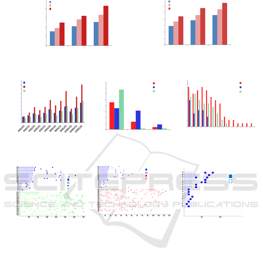
7 RESULTS
Figure 4 shows the latency and the number of pack-
ets transmitted to complete the scheduling when sim-
ulated with TOSSIM. In Figure 4(a), the average la-
tency is shown. We can see that the latency is low, al-
though EECF considers contiguousness of slots. Also
we see that the latency is directly related to the neigh-
borhood size/network density. Figure 4(b) shows the
average number of packet transmissions per node to
complete the scheduling. From the figure we see that
it increases linearly as the neighborhood size/network
density increases.
As expected, in general, the algorithms that use
the shortest path as a backbone show good results.
From the figure 5(a) we can see that the latencies of
EECF and SP-DAS can be two times lower than that
of 2DAS. The figure 5(b) shows the number of chil-
dren of networks constructed by EECF, SP-DAS and
2DAS. As can be observed, 2DAS has more nodes
that have large number of children, which implies that
nodes in 2DAS should be awake more time slots than
EECF and SP-DAS.
Figures 6(a) and 6(b) show the transmission and
reception time slots of the 15 nodes of EECF, 2DAS
and SP-DAS with the maximum number of slots.
From the figure we can see that EECF’s reception
slots are contiguous while 2DAS’s and SP-DAS’s re-
ception slots are usually separated. It can also be ob-
served that the nodes scheduled with EECF needs to
SENSORNETS 2016 - 5th International Conference on Sensor Networks
84

0
50
100
150
200
250
400 600 800
Latency
Number of nodes
Radius = 10m
Radius = 15m
Radius = 20m
(a) The average latency.
0
10
20
30
40
50
60
70
400 600 800
Number of packets
Number of nodes
Radius = 10m
Radius = 15m
Radius = 20m
(b) The number of packet transmissions per node.
Figure 4: The average latency and number of packet transmissions with different network sizes (EECF).
0
50
100
150
200
250
300
350
400
450
500
Latency (slots)
Network size (transmission range)
EECF
2DAS
SP-DAS
(a) The latencies with different network sizes and
transmission ranges
0
50
100
150
200
250
300
350
400
0 1 2
Number of nodes
Number of children
2DAS
EECF
SP-DAS
(b) The number of nodes with 0,1 and 2 children.
0
2
4
6
8
10
12
14
3 4 5 6 7 8 9 10 11 12 13 14 15 16 17
Number of nodes
Number of children
2DAS
EECF
SP-DAS
(c) The number of nodes with ≥3 children.
Figure 5: Comparison of EECF, SP-DAS and 2DAS.
Number of slots per node
Slot number
EECF Tx slot
EECF Rx slot
SP-DAS Tx slot
SP-DAS Rx slot
(a) The number of slots per node
Number of slots per node
Slot number
EECF Tx slot
EECF Rx slot
2DAS Tx slot
2DAS Rx slot
(b) The number of slots per node
Slot number
Number of slots per node
EECF Tx slot
EECF Rx slot
(c) The number of slots per node
Figure 6: (a) and (b)Comparison of EECF, SP-DAS and 2DAS (400 nodes, transmission range=15m), (c) Testbed results.
switch from the sleep to the active mode at most 3
times. While in 2DAS and SP-DAS the number of
switches could be large and can alternate every slot.
From the figure we can see that in SP-DAS and 2DAS
the maximum number of switches is 13 and 20 respec-
tively. This shows that EECF is more energy efficient
as nodes in EECF should be awake fewer time slots
and make fewer sleep-active switches. Figure 6(c)
shows the results obtained from the testbed experi-
ments which confirm that the algorithm assigns con-
tiguous slots to nodes.
As EECF and SP-DAS use a shortest path in their
aggregation tree, the number of nodes with 2 trans-
mission slots are equal. However, in the figure, there
are 9 nodes in EECF and only 7 nodes in SP-DAS
with 2 transmission slots. It is because in SP-DAS
there could be nodes that have more children than that
of the nodes on the shortest path. From the figure 5(a)
we can also see that, in general, SP-DAS has a bit
lower latency than EECF.
8 CONCLUSION
In this paper, we proposed two algorithms that bal-
ance energy consumption among nodes and sched-
ule data aggregation. We proved a number of theo-
retical results and the correctness of the algorithms.
Experimental results showed the performance of the
algorithms, and supported the correctness of our al-
gorithms. To the best of our knowledge, this is the
first work that deal with the data aggregation schedul-
ing problem in WSNs with more than one sink where
many nodes send data to many sinks.
Towards Energy-efficient Collision-free Data Aggregation Scheduling in Wireless Sensor Networks with Multiple Sinks
85

ACKNOWLEDGEMENTS
This work has been funded in part by the Committee
of Science of the Ministry of Education and Science
of the Republic of Kazakhstan through the program
N0.0662 “Research and development of energy effi-
ciency and energy saving, renewable energy and en-
vironmental protection for 2014 - 2016”.
REFERENCES
Akyildiz, I. F., Su, W., Sankarasubramaniam, Y., and
Cayirci, E. (2002). Wireless sensor networks: a sur-
vey. Computer Networks, 38(4):393–422.
Akyildiz, I. F. and Vuran, M. C. (2010). Wireless Sensor
Networks. John Wiley and Sons, Ltd.
Bo, Y. and Li, J. (2011). Minimum-time aggregation
scheduling in multi-sink sensor networks. In SECON,
pages 422–430. IEEE.
Doddavenkatappa, M., Chan, M. C., and Ananda, A. L.
(2011). Indriya: A low-cost, 3d wireless sensor net-
work testbed. In TRIDENTCOM, volume 90, pages
302–316. Springer.
Gilbert, E. N. and Pollak, H. O. (1968). Steiner minimal
tree. SIAM Journal on Applied Mathematics, 16:1–
29.
Hui Zhou, Dongliang Qing, X. Z. H. Y. and Xu, C. (2012).
A multiple-dimensional tree routing protocol for mul-
tisink wireless sensor networks based on ant colony
optimization. 2012.
Jhumka, A. (2010). Crash-tolerant collision-free data ag-
gregation scheduling for wireless sensor networks. In
SRDS 2010, pages 44–53.
Jolly, G. and Younis, M. (2005). An energy-efficient, scal-
able and collision-free mac layer protocol for wire-
less sensor networks. Wirel. Commun. Mob. Comput.,
5(3):285–304.
Karp, R. M. (1972). Reducibility among combinatorial
problems. In Proceedings of a symposium on the Com-
plexity of Computer Computations, pages 85–103.
Kawano, R. and Miyazaki, T. (2008). Distributed data ag-
gregation in multi-sink sensor networks using a graph
coloring algorithm. AINA, pages 934–940.
Lee, H., Klappenecker, A., Lee, K., and Lin, L. (2005).
Energy efficient data management for wireless sensor
networks with data sink failure. IEEE MASS, 0:210.
Levis, P., Lee, N., Welsh, M., and Culler, D. (2003). Tossim:
accurate and scalable simulation of entire tinyos appli-
cations. In SenSys ’03, pages 126–137.
Mottola, L. and Picco, G. P. (2011). Muster: Adaptive
energy-aware multisink routing in wireless sensor net-
works. IEEE Trans. Mob. Comput., 10(12):1694–
1709.
Rajendran, V., Garcia-Luna-Aveces, J., and Obraczka, K.
(2005). Energy-efficient, application-aware medium
access for sensor networks. In Mobile Adhoc and Sen-
sor Systems Conference, 2005, pages 8 pp.–630.
Rajendran, V., Obraczka, K., and Garcia-Luna-Aceves, J. J.
(2006). Energy-efficient, collision-free medium ac-
cess control for wireless sensor networks. Wirel.
Netw., 12(1):63–78.
Shih, E., Calhoun, B., Cho, S., and Chandrakasan, A.
(2001). Energy-efficient link layer for wireless mi-
crosensor networks. In VLSI, 2001. Proceedings.
IEEE Computer Society Workshop on, pages 16–21.
Sitanayah, L., Brown, K. N., and Sreenan, C. J. Multiple
sink and relay placement in wireless sensor networks.
In WAITS 2012.
Sohrabi, K., Gao, J., Ailawadhi, V., and Pottie, G. (2000).
Protocols for self-organization of a wireless sensor
network. Personal Communications, IEEE, 7(5):16–
27.
Thulasiraman, P., Ramasubramanian, S., and Krunz, M.
(2007). Disjoint multipath routing to two distinct
drains in a multi-drain sensor network. In INFOCOM,
pages 643–651. IEEE.
Tuysuz Erman, A. and Havinga, P. (2010). Data dissem-
ination of emergency messages in mobile multi-sink
wireless sensor networks. In Med-Hoc-Net 2010,
pages 1–8.
Valero, M., Xu, M., Mancuso, N., Song, W.-Z., and Beyah,
R. A. (2012). Edr
2
: A sink failure resilient approach
for wsns. In ICC 2012. IEEE.
Wan, P.-J., Alzoubi, K. M., and Frieder, O. (2004). Dis-
tributed construction of connected dominating set in
wireless ad hoc networks. Mobile Network Applica-
tions, 9(2):141–149.
Yu, B., Li, J., and Li, Y. (2009). Distributed data aggrega-
tion scheduling in wireless sensor networks. In 28th
IEEE International Conference on Computer Commu-
nications, Joint Conference of the IEEE Computer and
Communications Societies, 19-25 April 2009, Rio de
Janeiro, Brazil, INFOCOM, pages 2159–2167.
SENSORNETS 2016 - 5th International Conference on Sensor Networks
86