Low Order Aberrations Compensation by Direct Adjustment
of the Reflective Beam Shaper in Slab Laser
Liu Wenguang
1
, Zhou Qiong
1
, Wang Gang
2
, Xie Kun
1
, Yan Baozhu
1
and Xi Fengjie
1
1
College of Opto-electronic Science and Engineering, National university of Defense Technology,
Changsha, Hunan, China
2
Science and Technology on Solid-State Laser Laboratory, Beijing, China
Keywords: Slab Laser, Low Order Aberrations, Compensation, Beam Shaper.
Abstract: A direct method for compensation of low order aberrations with large PV value was presented in this paper.
In which, the relationship between the optical layout parameters and the output aberration coefficients were
derived by ray matrix method. Then, the adjustment parameters calculated by the equations were used to
change the optical layout parameters to compensate the low order aberrations with defocus and astigmatism.
The effectiveness of this method was verified by simulations based on the optical models built in a optical
design software. It shows that the low order aberrations can be accurately compensated to a level below 0.5λ
by the direct method.
1 INTRODUCTION
In the development of high power slab lasers, both
output power and beam quality are crucial parameters
to be considered. Although power scaling of slab laser
can be realized by MOPA (Master Oscillator and
Power Amplification) configuration, preserving high
beam quality in high power slab laser is a real
challenge (Redmond et al, 2007). In high power slab
lasers, the Peak-Valley (PV) value of thermally
induced wave-front distortion can be dozens of
micrometers (Ganija et al., 2013), and it’s difficult to
be corrected by a deformable mirror with limited
correction range (typically in the range of 6 μm).
Multiple deformable mirrors are proposed to correct
the wave-front distortions in high power lasers (Xiang
et al., 2012; Conan et al., 2007). However, this
solution is both expensive and complex. Some
experiments have been done to analysis the
characteristics of the wave-front in the high power
slab laser (Liujing et al., 2011)
.
It shows that in the
distortions, low order aberrations, mainly consist of
defocus and astigmatism, are the main contributors.
So the two-steps beam cleanup concept is proposed
as a cost-effective approach to get high beam quality.
That is, low order aberrations are compensated by one
compensator firstly. And next, the high order
aberrations are corrected by one deformable mirror.
Static phase corrector (W Qiao, et al, 2014) can be
used to compensate some low order aberrations, but
it doesn’t work well when the operational conditions
were changed, and it can also be thermally distorted
under high power flux. A reflective beam shaper with
two cylindrical mirrors and one spherical mirror was
proposed to compensate the low order aberrations by
active adjustment of the optical parameters with PID
algorithm (Wenguang et al., 2014). Due to the
respond speed of the motorized linear stage used, the
convergence of PID controller may take about 20s.
In this paper, for the purpose of speeding the
compensation process of low order aberrations in slab
laser, a direct method was proposed, in which the
relationships between the low order aberrations and
adjusting parameters were derived from ray matrix
equations. Simulations were done to verify the
correctness of the method.
2 THEORITICAL DERIVATION
2.1 Layout of the Reflective Beam
Shaper
A reflective beam shaper is often used to transform a
narrow beam to a square one in slab laser system. The
beam shaper can also be used to compensate the low
Wenguang, L., Qiong, Z., Gang, W., Kun, X., Baozhu, Y. and Fengjie, X.
Low Order Aberrations Compensation by Direct Adjustment of the Reflective Beam Shaper in Slab Laser.
DOI: 10.5220/0005736501130118
In Proceedings of the 4th International Conference on Photonics, Optics and Laser Technology (PHOTOPTICS 2016), pages 115-120
ISBN: 978-989-758-174-8
Copyright
c
 2016 by SCITEPRESS – Science and Technology Publications, Lda. All rights reserved
115

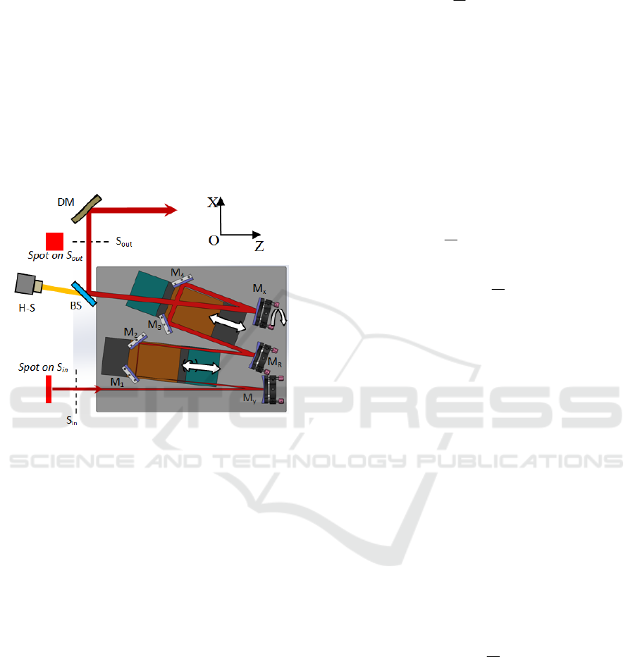
order aberrations, As shown in Fig.1, where the beam
shaper mainly consists of two cylindrical mirrors(y-
oriented mirror M
y
, x-oriented mirror M
x
), one
spherical mirror (M
R
). The distance between M
y
and
M
R
is L
1
, and the distance between M
R
and M
x
is L
2
.
Four plane mirrors (M
1
, M
2
, M
3
, M
4
) are used to fold
the optical path, for the purpose of keeping the output
beam position unchangeable while L
1
and L
2
are
adjusted to compensate the defocus and 0 degree
astigmatism, and M
x
can be rotated a angle of κ
about z-axis to compensate the 45 degree astigmatism.
The PID algorithm was used to adjust L
1
and L
2
,and
κ to slowly compensate the low order aberrations.
Figure 1: The optical layout of a reflective beam shaper and
adjustment parameters for compensation of low order
aberrations.
2.2 Matrix Analysis of the Low Order
Aberration Compensator
In this paper, matrix methods are used to analyze the
relationship between low order aberrations and the
adjustment of L
1
and L
2
,and κ， to compensate the
aberrations directly and quickly without PID
algorithm.
Ray tracing are taken from M
y
to the output plane
S
out
, as shown in Fig.1. Using a Cartesian-azimuth
representation, an incident ray on M
y
can be written
as:
in
x
V
y
α
β






=






(1)
For a reflective y-oriented cylindrical mirror of
curvature R
1
the matrix is:
1
1000
2
-100
0010
0001
cy
R
M






= 








(2)
The propagation matrix between M
x
and M
R
is ：
1
1
1
1L 0 0
0100
001
0001
L
M
L






=






(3)
The reflective matrix of spherical mirror M
R
of
curvature R
2
is:
2
2
1000
2
100
0010
2
00 1
R
R
M
R






−


=






−




(4)
The propagation matrix between M
R
and M
x
is :
2
2
2
1L 0 0
0100
001
0001
L
M
L






=






(5)
The coordinate transform matrix with rotation angle
of κ about z-axis is:
cos 0 -sin 0
0cos 0-sin
sin 0 cos 0
0sin 0cos
z
R
κκ
κκ
κκ
κκ






=






(6)
For a reflective x-oriented cylindrical mirror of
curvature R
3
the matrix is:
3
1000
01 0 0
00 1 0
2
00- 1
cx
M
R







=








(7)
And the coordinate transform matrix with rotation
angle of -κ about z-axis is:
cos 0 sin 0
0cos 0sin
sin 0 cos 0
0sin0cos
zp
R
κκ
κκ
κκ
κκ






=


−


−


(8)
The propagation matrix between M
y
and S
out
is :
PHOTOPTICS 2016 - 4th International Conference on Photonics, Optics and Laser Technology
116

3
3
3
1L 0 0
0100
001
0001
L
M
L



=



(9)
Matrix of reflective beam shaper in this paper can be
calculated by the matrix product of the component
matrixes:
321
L
zp cx z L R L cy
M
MRMRMMMM=⋅⋅⋅⋅⋅⋅⋅
(10)
2.2.1 Functions for Compensating the
Defocus and 90
O
Astigmatism
In Cartesian coordinates, the combination of defocus
and 90
o
astigmatism can be written as:
22
(, )
22
x
y
x
y
wxy
R
R
=+
(11)
where R
x
is the curvature of beam divergence in
XOZ plane, and R
y
is the curvature in YOZ plane
(Geovanni et al., 2014). So the ray incident M
y
with
defocus and 90
o
astigmatism in matrix form is:
=
x
in
y
x
x
x
w
R
x
V
y
y
w
y
y
R






∂





∂

=








∂




∂



(12)
Rewrite the distance as
()
112 1
R2
L
RL=+ +Δ
()
223 2
R2
L
RL=+ +Δ
where ΔL
1
and ΔL
2
are the adjustment of distance
desired to compensate the defocus and 90
o
astigmatism. Set rotation angle κ=0 for the
simplification of derivation, The rays leaving M
x
is
calculate by
'
'
=
'
'
out in
x
VMV
y
α
β



=⋅=



()( )()
()
()()
2
2222
13 1 2 1 3 1 1 2
12 2 1 3 1 3
12 12
2
11 1
12
2
222 2
1313 1 13231
32 13 3 2 3
23 23
2
21
242L22 L
22
2
22
-
22 222
22
2
-2
xx x
x
x x
x
x
yy
y
y y
RRR R R R RL LR
RR RR RR RL
xx
RRR RRR
RRRL
x
RRR
RR RLR R R LLLRL
RR RR R R R L
y
y
RRR RRR
RR
 −+−Δ−−  Δ− Δ
−−−

+
+−Δ

−− Δ + + +Δ Δ− Δ
−− −

+
++
()
212
23
24
y
y
RL LL
y
RRR
 
 
 
 
 
 
 
 
 
 
 
 
Δ+ΔΔ
 
 
 
(13)
From Eq. (13) the adjustment of distance ΔL
1
and
ΔL
2
are obtained when
'0,'0 α
β
==
:
2
1
1
1
2(2 )
x
R
L
R
R
Δ=
−
(14)
2
2
2
11
22 + 2
y
R
L
R
RL
Δ=


+Δ


(15)
It means that defocus and 90
o
astigmatism can be
compensated by proper adjustment of ΔL
1
and ΔL
2
.
However, in the practical compensation process,
Wave-front aberrations on S
out
are often expressed as
Zernike coefficients in most wave-front sensor, such
as Hartman-Shack sensors. So it is convenience to
express ΔL
1
and ΔL
2
as the functions of Zernike
coefficients detected by H-S sensor on output plane
S
out
.
Before adjustment, ΔL
1
=0, ΔL
2
=0. From Eq. (13),
the relationship of x-curvature of divergence beam on
the output plane R
x
’ and the curvature on the input
plane R
x
is:
2222
12 2 1 3 1 3
2
1
22
x'
'= =-
'2
x
x
RR RR R R R L
R
R
α
−−−
(16)
We can rewrite Eq. (16) as:
2222
1121313
2
2
2' 2
=
2
x
x
R
RRR RR RL
R
R
+−−
(17)
In the same manner, the relationship of y-
curvature of divergence beam on the output plane R
y
’
and the curvature on the input plane R
y
is:
2222
2323123
2
3
2' 2
=
2
y
y
RR RR RR RL
R
R
+−−
(18)
The relationship between Zernike coefficients
and beam divergence curvature on the output plane
S
out
is:
()
2
0
46
'
2
223 6
x
x
rk
R
ZZ
η
λ
==
−
(19)
()
2
0
46
'
2
223 6
y
y
k
r
R
ZZ
η
λ
==
+
(20)
Where
2
0
r
η
λ =
,
()
x
46
k=1 2 3Z 6Z−
()
y46
k=1 23Z+ 6Z
r
0
is the normalized aperture on the output plane, and
λ is the wavelength used in the beam shaper, Z
4
is the
Low Order Aberrations Compensation by Direct Adjustment of the Reflective Beam Shaper in Slab Laser
117

Zernike coefficient of defocus term, and Z
6
is the
coefficients of 90
o
astigmatism defined in the wave-
front sensor. Insert Eq. (17)~(20) into Eq. (14) and
Eq. (15), adjustment of distance ΔL
1
and ΔL
2
can be
determined according to the Zernike coefficients
from wave-front sensor on output plane:
()
2
2
1
33
22
x
R
L
kR L
η
Δ=
−−
(21)
()
2
3
2
22
33 132
222/
y
R
L
kRL LRR
η
Δ=

+−+Δ

(22)
2.2.2 Functions for Compensating the 45
O
Astigmatism
In Cartesian coordinates, the 45
o
astigmatism can be
written as:
2
(, )
c
wxy xy
R
=
(23)
where R
c
is the curvature parameter of 45
o
astigmatism
[9]
.
So the ray incident M
y
with 45
o
astigmatism in
matrix form is:
45
2
2
c
in
c
x
x
y
R
V
yy
x
R
α
β











==













(24)
The rays leaving S
out
can be calculate by
45 45out in
VMV=⋅
In the derivation of V
out45
, both ΔL
1
and ΔL
2
is set
to zeros for the simplicity of derivation, and the terms
of sin
2
κ are omitted for it’s a high order quantity in
the functions. The rays leaving S
out
can be written as:
2
13 2
2
3
12
22
13 2 1
23 2
45
2
3132
3
22
22
212132
13 23
'
'
sin(2 )- sin(2 ) sin(2 ) 2 cos
+
'
'
'
'
sin 2 2 cos sin 2 sin 2
c
c
cc
out
c
c
cc
RR RR
xyL
RRR
x
RR R R R
xy
RRR RR
V
y
RRRR
yxL
RRR
RR RR RR R
xy
RRR R RR
α
κκ κ κ
α
β
β
κκ κκ

−
−− +



−





==


−

−− +




−−

+












(25)
(24)
The rotation of M
x
with an angle of κ is to
eliminate the 45
o
astigmatism, that is, the terms about
y in
' α
become zeros, and the terms about x in
'
β
also become zeros by proper rotating of M
y
with an
angle of κ. From Eq. (25), we can derive the
relationship between rotation angle κ and the input
45
o
astigmatism parameter R
c
:
1
tan
c
R
R
κ =
(26)
When κ is a small angle
1
sin tan
c
R
R
κκ ==
(27)
Insert Eq. (26) into Eq. (25), we can found that after
the 45
o
astigmatism is compensated, there still are
some small defocus:
()
2
1132
2
23
-
'=2
c
RRRR
x
RRR
α
(28)
()
2
113 2
2
23
'2
c
RRR R
y
RRR
β
−
=
(29)
In most situations, the defocus introduced is small
enough that could be omitted, and also it can be
compensated by adjusting of L
1
and L
2
later if it is
necessary.
The relationship between the coefficient of 45
o
astigmatism on the input plane and output plane can
be derived when we let κ=0:
1
3
'
cc
R
R
R
R
=
(30)
The relationship between the Zernike coefficient Z
5
and
'
c
R
is:
2
0
5
1
'
6Z
cxy
r
R
k
η
λ
==
(31)
Where
()
5
16
xy
kZ=
Insert Eq. (30) and Eq. (31) into Eq. (26), the equation
between the rotation angle κ and the Zernike
coefficient of 45
o
astigmatism on the output plane can
be derived as:
3
tan
x
y
R
k
κ
η
=
(32)
From Eq. (32), we can find that the rotation angle κ
have a very simple linear relationship with the
Zernike coefficient Z
5
on the output plane.
PHOTOPTICS 2016 - 4th International Conference on Photonics, Optics and Laser Technology
118

3 VERIFICATION OF THE
METHOD
In the derivation of the relationships between the
compensating parameters (ΔL
1
, ΔL
2
, κ) and the
Zernike coefficients (Z
4
,Z
5
,Z
6
) on the output plane,
some higher order quantities have been omitted. To
verify the correctness of the theoretical derivation,
the optical model of the reflective beam shaper
designed in Sec.2 was built in commercial optical
design software, where R
1
=516mm ， R
2
=800mm ，
R
3
=206mm ， L
1
=(R
1
+R
2
)/2, L
2
=(R
2
+R
3
)/2. In the
model, the input aberrations were generated by
adding a phase plate with different combination of
Zernike coefficients. And the Zernike coefficients of
aberrations on the output plane and normalized radius
r
0
can be generated by the commercial software, to
serve as the H-S sensor in Fig.1, which is needed in
Eq. (21), (22) and (31). In the calculations of the
adjusting parameters, the rotational angle κ was the
first parameter to be calculated, then the adjustment
of distance ΔL
1
was calculated, at last, ΔL
2
was
calculated. After κ, ΔL
1
and ΔL
2
were calculated,
these value were sent to the optical model, then the
wave-front parameters, such as Zernike coefficients
and Peak-to valley (PV) of the wave-front can be
generated by the software. The comparison before
and after compensation by adjusting of κ, ΔL
1
and ΔL
2
for four cases of input low order aberrations are listed
in Table.1.
It shows that the adjusting parameters calculated
in case1~case3 are very well to compensate the low
order aberrations in the input plane, and the PV value
after compensation is below 1λ, which is suitable for
later wave-front corrections by a higher order
deformable mirror, as shown in Fig. 1.
When the aberrations consists of both defocus
and 45-Deg astigmatism, the first step of adjusting
values of ΔL
1
and ΔL
2
are less effective, and the PV
value after compensation is still larger than 1λ, as
shown in Fig.2(h). It is because the adjusting of 45-
Deg astigmatism can introduce small defocus, as
illuminated in Eq. (27) and Eq. (28). So two steps
compensation are necessary to solve this problem.
That is, after the first step compensation, the
normalized radius and Zernike coefficients are
renewed to serve as the calculating parameters for
second step compensation, as listed in case 4b in
Table.1. Then the second adjusting parameters are
obtained, and the final compensation result is
satisfactory with a wave-front PV of 0.31λ.
Table 1: Compensation results for 4 cases.
Optical parameters on S
out
before compensation
Adjusting parameter
and PtV after
compensation
r
0
/mm
Z
4
Z
5
Z
6
PV
i
/λ
ΔL
1
/mm
ΔL
2
/mm
κ
Deg
PV
/λ
1 6.15 1.14 0 1.60 4.18 0.27
5.08
0 0.31
2 9.85 2.37 0 -3.33 8.53
67.0
0 0 0.24
3 5.70 0.02 0.52 0.01 2.53 -0.14 0.06 0.47
0.47
4a 7.30 3.25 0.79 3.35 13.3 22.3 9.6 0.45 1.13
4b 6.45 0.25 0 0.16 1.13 3.9 0.68 0 0.31
4 Total adjusting parameters for case 4
26.2
10.3 0.45
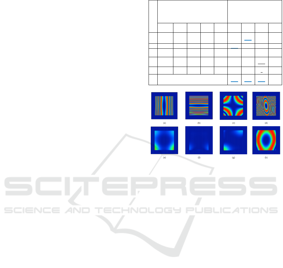
Figure 2: Wave-front distribution before compensation (a)
PV=4.18λ, in case 1, (b) PV=8.53λ, in case2, (c) PV=2.53λ,
in case3, (d) PV=13. 3λ, in case4 and after low order
aberration compensation (e) PV=0.31λ, (f) PV=0.24λ, (g)
PV=0.43λ, (h) PV=1.13λ (0.31λ after two steps
compensation).
4 CONCLUSIONS
Based on the relationships between the optical layout
parameters of a reflective beam shaper and Zernike
coefficients on the output plane, the low order
aberrations can be well compensated by directly
adjusting the parameters. And the PV value after
compensation is below 1λ, which can be further
corrected by deformable mirrors. With this direct
compensation method, low order aberration with
large PV value in slab laser could be compensated
both efficiently and quickly.
ACKNOWLEDGEMENTS
This work was supported by Science and Technology
on Solid-State Laser Laboratory Foudation
(No.9140C040101140C04016) and National Natural
Science Foundation of China (NSFC, No.61379065
and No.11504423).
Low Order Aberrations Compensation by Direct Adjustment of the Reflective Beam Shaper in Slab Laser
119

REFERENCES
S. Redmond, S. McNaught, J. Zamel, et al, 2007. 15 kW
near-diffraction-limited single-frequency Nd:YAG
laser, OSA/CLEO.
M. Ganija, D. Ottaway, P. Veitch, et al, 2013. High power,
near diffraction limited, Yb: YAG slab laser, Opt.
Express.
L Xiang, W Shuai, H Yang, et al, 2012. Double-
deformable-mirror adaptive optics system for laser
beam cleanup using blind optimization, Opt. Express.
R. Conan. C. Bradley, P. Hampton, O. Keskin, et al. 2007.
Distributed modal command for a two deformable-
mirror adaptive optics system, Appl. Opt.
X Liujing, Y Ping, L Xinbo, et al, 2011. Application of
Hartmann-Shack wavefront detector in testing distorted
wavefront of conduction cooled end-pumped slab laser,
Chin. J. Lasers.
W Qiao, Zh Xiaojun, W Yonggang, S Liqun, et al, 2014. A
simple method for astigmatic compensation of folded
resonator without Brewster window, Opt. Express.
L Wenguang, Zh Qiong, F Fei, et al, 2014. Active
compensation of low-order aberrations with reflective
beam shaper, Opt. Engineering.
H. J. Geovanni, M. J. Zacarías and M. H. Daniel, 2014.
Hartmann tests to measure the spherical and
cylindrical curvatures and the axis orientation of
astigmatic lenses or optical surfaces, App. Optics.
PHOTOPTICS 2016 - 4th International Conference on Photonics, Optics and Laser Technology
120