Forecast-augmented Route Guidance in Urban Trafﬁc Networks based

on Infrastructure Observations

Matthias Sommer, Sven Tomforde and J

org H

ahner

University of Augsburg, Organic Computing Group, Augsburg, Germany

Keywords:

Trafﬁc Guidance, Proactive Vehicle Routing, Time Series Forecasting, Organic Trafﬁc Control.

Abstract:

Increasing mobility and raising trafﬁc demands lead to serious congestion problems. Intelligent trafﬁc manage-

ment systems try to alleviate this problem with optimised signalisation of trafﬁc lights and dynamic route guid-

ance (DRG). One solution for the former aspect is Organic Trafﬁc Control (OTC), offering a self-organised,

decentralised trafﬁc control system. Based on OTC, this paper presents two proactive routing protocols, re-

sembling techniques known from the Internet domain, applied to the trafﬁc routing problem: Distance Vector

Routing and Link State Routing. These protocols were adapted to utilise forecasts of trafﬁc ﬂows to offer

anticipatory and time-dependant DRG for road users. The efﬁciency of these protocols is demonstrated with

simulations of two Manhattan-type road networks under disturbed and undisturbed conditions. The results

indicate their beneﬁt in terms of lower travel times and emissions, even under low compliance rates.

1 INTRODUCTION

Trafﬁc congestion is a serious problem affecting all

trafﬁc participants. The resulting waste of time and

fuel leads to billions of dollars lost annually

. Ur-

ban road networks come to their capacity limit due to

increasing demands. The complexity of these trafﬁc

control systems, due to mutual inﬂuence of different

trafﬁc control strategies, is not longer feasible for a

central instance. Thus, decentralised, self-organising

and self-optimising approaches, that better utilise the

existing infrastructure are needed. Organic Trafﬁc

Control (OTC) (Prothmann et al., 2011) represents

such an approach. OTC selects the best known phase

durations at intersections depending on the current

trafﬁc ﬂow while learning the impact of its decision to

improve the signalisation behaviour over time. OTC

extends the existing trafﬁc light controllers (TLC) at

intersections via the Observer/Controller architecture

(Tomforde et al., 2010). By communicating the lo-

cal delays (i.e. occurring at the underlying intersec-

tion) and estimated travel times to nearby intersec-

tions, TLCs have the ability to determine the short-

est paths to prominent destinations (such as the main

hall or the main station) based on the current trafﬁc

ﬂows within the network. The beneﬁts of dynamic

Urban mobility report, http://mobility.tamu.edu/ums/

(last access: 2016-02-02)

route guidance (DRG) systems are the alleviation of

congestion, the enhancement of the performance of

the road network, and the provision of navigational

assistance for travellers which are unfamiliar with the

network (Dong, 2011).

Routing protocols compute the fastest or shortest

route from a starting point to a destination. This cal-

culation is typically based on static information or re-

cently monitored trafﬁc data. The computed routes

may then be visualised via Variable Message Signs

(VMS) or on a navigational system and give drivers

an indication how to traverse the network to reach

their destination as fast as possible. This approach

yields signiﬁcant problems: First, the drivers need

time to follow their proposed route. The trafﬁc sit-

uation might have changed and so, the routes might

be outdated. This leads to repeated re-routings, de-

creasing the acceptance of the route guidance mech-

anism. Second, especially in situations with devel-

oping congestion, a fast reaction is valuable to avoid

further negative impacts on the trafﬁc. Forecasts of

the future trafﬁc ﬂow patterns help to detect capacity

shortages in advance.

This paper presents two novel, anticipatory and

time-dependent route guidance protocols for usage

in the infrastructure: Temporal Link State Rout-

ing (TLSR) and Temporal Distance Vector Rout-

ing (TDVR). These protocols are used to distribute

Sommer, M., Tomforde, S. and Hähner, J.

Forecast-augmented Route Guidance in Urban Trafﬁc Networks based on Infrastructure Observations.

In Proceedings of the International Conference on Vehicle Technology and Intelligent Transport Systems (VEHITS 2016), pages 177-186

ISBN: 978-989-758-185-4

177

knowledge about forecasts of the trafﬁc ﬂow for sev-

eral future time steps in combination with current

route states. Thereby, both concepts extend Distance

Vector Routing (DVR) and Link State Routing (LSR)

that were adapted for urban road networks (Proth-

mann et al., 2012) which just consider the current

trafﬁc conditions. Furthermore, the learning forecast

module within the OTC system is presented which al-

lows for proactive adaptation to upcoming changes in

trafﬁc demand. The major goals are the improvement

of the network’s robustness and the minimisation of

the average travel time and emissions by preventing

congestion. A better distribution of the trafﬁc streams

allows to use the capacity of the road network more

efﬁciently. The performance of the novel protocols

is investigated in a simulation-based evaluation with

two artiﬁcial networks under free ﬂow and disturbed

conditions. The considered disturbances are due to

high trafﬁc demands and incidents modelled as abrupt

blockages. The evaluation results indicate that proac-

tive route guidance lowers the overall travel times and

delays for road users. The algorithms are evaluated

with several compliance rates (i.e. the degree to which

drivers follow the route recommendations), showing

the beneﬁt of our approach even under low compli-

ance rates.

The remainder of this paper is structured as fol-

lows: Section 2 presents a short overview of the state

of the art in DRG in urban road networks. Section 3

brieﬂy introduces the OTC system and its main com-

ponents. The routing component and the new rout-

ing protocols are discussed in Section 4. Section 5

presents the evaluation results. The paper concludes

with an outlook to future work in Section 6.

2 STATE OF THE ART

Research in the ﬁeld of vehicular route guidance can

be categorised in a variety of ways (Schmitt and Jula,

2006). The routes can be computed in a static or in

a dynamic fashion. First, static methods compute a

ﬁxed route before the start of the trip. Today, many

cars come equipped with on-board GPS-based navi-

gation systems (such as Garmin or TomTom) (Kaplan,

2005). The navigation relies on installed maps of the

network which are mostly used by modiﬁed versions

of the Dijkstra (Dijkstra, 1959) or the A* algorithm

(Hart et al., 1968). They are applied to ﬁnd the short-

est route for a given starting point and a ﬁxed destina-

tion (Prothmann et al., 2012; Nannicini et al., 2012).

Dong (Dong, 2011) presents a brief summary of the

published literature on in-vehicle route guidance sys-

tems until 2010. Second, reactive routing protocols

also compute a route upfront. This can be subject to

change during the trip, depending on the real-time in-

formations received. The protocol reacts to chang-

ing trafﬁc conditions and computes a new route based

on these information. Third, predictive routing proto-

cols go one step further. Apart from reacting to the

current situation, but furthermore, they generate fore-

casts of the upcoming trafﬁc streams and incorporate

those forecasts into the computation of the proposed

route. It was shown that reactive protocols and espe-

cially predictive approaches lower the average travel

time in urban road networks (Fu, 2001), whereas re-

active protocols are less complex than predictive sys-

tems, at the cost of decreased robustness against inci-

dents and congestion (Schmitt and Jula, 2006).

Furthermore, DRG systems can be divided into

centralised an decentralised approaches. A study of

decentralised strategies for route guidance (F.S. Zu-

urbier and van Zuylen, 2006), comparing centralised

an decentralised systems, points out that decentralised

approaches have lower computational complexity, are

easily scaled and extended, while being more robust

against failures and measurement errors than cen-

tralised systems, but might only come up with a sub-

optimal system-wide solution. In a centralised sys-

tem, all data is gathered in a trafﬁc management cen-

tre where route proposals are computed for the entire

network, taking into account system-wide objectives.

SACaNT-CNV (Simulation of Anticipatory Net-

work Vehicle Trafﬁc - Convergence) is a decen-

tralised, proactive route guidance system (Wunder-

lich et al., 2000). Equipped vehicles are routed on a

next-hop basis, each vehicle having a compliance rate

of 100% (i.e. strictly following the proposed route).

Non-equipped vehicles are assumed to statically fol-

low the shortest free-ﬂow routes. To determine the

route proposals, time-dependent link travel times are

used in a trafﬁc simulation. It was shown that this

approach leads to faster travel times for equipped ve-

hicles.

(Dong et al., 2006) propose a user-equilibrium

time-dependent trafﬁc assignment algorithm, using

the simulation assignment model DYNASMART.

They estimate the current trafﬁc conditions and derive

short-term road utilisations to forecast travel times.

Their results indicate that this route guidance strategy

may reduce the total trip time.

Other decentralised approaches rely on car-2-car

communication based on ﬂoating car data. A modi-

ﬁed version of the Internet routing protocol BeeHive

(Horst F. Wedde et al., 2007) resulting in the BeeJamA

protocol routes trafﬁc participants on a next-hop basis

from intersection to intersection. Navigation servers

store and manage regional routing tables with routes

VEHITS 2016 - International Conference on Vehicle Technology and Intelligent Transport Systems

178

to other areas. These entries are updated based on data

sent by vehicles that are assumed to repeatedly trans-

mit their position, speed and destination. OTC does

not demand additional hardware in vehicles and elim-

inates the single point of failure of a central server

with a decentralised approach.

A delegate multi-agent system based on ant be-

haviour was presented in (Claes et al., 2011). It rep-

resents a decentralised approach for anticipatory ve-

hicle routing. Every vehicle has to be equipped with a

smart device, depicting the vehicle agent that gathers

data from the vehicle, such as its state and location,

and transmits these to infrastructure agents along the

road and to nearby vehicle agents. The vehicle agents

use this information to forecast road occupancies to

determine the best route to their destination.

In contrast to some of the previous approaches, the

DRG mechanism proposed in this paper does not rely

on equipped vehicles. The ﬂow and the signalisation

data are available at the responsible TLC (e.g. via

loop detectors or video cameras), representing a de-

centralised and proactive approach.

3 ORGANIC TRAFFIC CONTROL

Current trafﬁc management systems usually rely on

ﬁxed-time signal plans. Thus, they are not able to

adapt to the highly dynamic trafﬁc patterns and to re-

act to unforeseen situations, leading to longer travel

times and higher emissions. OTC (Prothmann et al.,

2011) extends parametrisable ﬁxed-time controllers,

offering a self-adapting, self-optimising system that

transfers the traditional design-time decisions to run-

time. OTC consists of four basic components: a)

adaptive control of trafﬁc lights, b) trafﬁc-dependent

establishment of Progressive Signal Systems, c) dy-

namic route guidance and d) forecasting of trafﬁc sit-

uations.

3.1 Adaptive Control of Trafﬁc Lights

OTC handles the adaptation of green times at trafﬁc

lights at intersections according to the present trafﬁc

conditions. The self-learning, self-optimising system

follows a safety-oriented concept that allows OTC to

adapt within certain controlled boundaries. Each in-

dividual instance of OTC is fully decentralised and

controls one intersection only. Fig. 1 depicts the Ob-

server/Controller architecture applied to trafﬁc con-

trol. The System under Observation and Control

(SuOC) situated at Layer 0 is a parametrisable ﬁxed-

time TLC. It offers interfaces for monitoring of detec-

tor data and adaptation of signal plans. The Observer

Layer 3

Layer 0

Control

signals

User

System under Observation

and Control (SuOC)

Layer 1

Parameter selection

Observer

Controller

Modified

XCS

Layer 2

Offline learning

Observer

Controller

Simulator

Collaboration mechanisms

Monitoring Goal Mgmt.

Detector

data

Figure 1: Architecture of an OTC-controlled TLC.

at Layer 1 retrieves raw data from the SuOC which

is processed in the following (e.g. ﬁlter noise or gen-

erate forecasts). This component provides a situation

description of the trafﬁc ﬂow of the intersection for

the corresponding Controller on Layer 1. This Con-

troller is represented by a learning classiﬁer system

with a database of rules (signal plans matched to situ-

ations). These are selected based on the current situa-

tion and actuated on Layer 0. Before a new signal plan

is added to the rule base, it is simulated and evaluated

based on an optimisation heuristic on Layer 2. The

simulator is conﬁgured with the topology of the inter-

section and the current trafﬁc situation. It evaluates

several signalisation plans based on an evolutionary

algorithm. The signal plan offering the lowest average

delay is returned to Layer 1. As simulations tend to be

time-consuming, Layer 2 acts in parallel to Layer 1.

At last, Layer 3 provides an interface for monitoring

and goal management. A more detailed description of

the process is given in (Prothmann et al., 2012).

3.2 Progressive Signal Systems

TLCs that are located at nearby intersections which

are directly connected via streets may communi-

cate with each other to form a distributed coordi-

nation of intersection controllers. Through this col-

laboration, Decentralised Progressive Signal Systems

(DPSS, also called ”green waves”) may be estab-

lished. The mechanism is a three-step-process: 1)

identiﬁcation of possible partners, 2) negotiation of

parameters and timing restrictions, and 3) establish-

ment of the DPSS for the most prominent streams

within the network (streams with the highest trafﬁc

ﬂows) leading to lower travel times while increasing

the throughput.

Forecast-augmented Route Guidance in Urban Trafﬁc Networks based on Infrastructure Observations

179

3.3 Dynamic Route Guidance

To turn OTC in an even more robust trafﬁc control

system, a self-organised route guidance mechanism

has been integrated that computes the fastest routes

through the network to prominent places based on the

current trafﬁc conditions. Techniques from the In-

ternet domain, such as the Distance Vector Routing

(DVR) and the Link State Routing (LSR) protocol

(Tanenbaum, 2002) were adapted to road trafﬁc guid-

ance (Prothmann et al., 2012). Since these protocols

work well for a complex network with a huge number

of nodes, such as the Internet, we see it as an appropri-

ate approach for urban road networks. TLCs use the

existing communication infrastructure to send their

locally monitored trafﬁc situations to nearby TLCs.

This situation description contains the turning delays

(approximated with a formula from (Webster, 1958),

Equation 1) and the estimated travel times for outgo-

ing sections (based on a formula from the U.S. Dept.

of Transportation (USDOT)

, Equation 2). Assum-

ing that M corresponds to the turning’s current trafﬁc

ﬂow in vehicles per hour, S denoting the saturation

ﬂow (the maximal ﬂow assuming permanent green),

representing the cycle time of the intersection and

denoting the turning’s effective green time, the turn-

ing’s delay is calculated as:

= 0.9 ∗ [

∗ (1 −t

)

2 ∗ (1 − M/S)

1800 ∗ g

M ∗ (1 − g)

] (1)

Finally, g =

∗S

corresponds to the degree of sat-

uration of the turning for the current green time and

trafﬁc ﬂow. The estimated travel time for a section is

computed in dependence of the monitored trafﬁc ﬂow

M as:

= t

∗ (1 + (M/C)

) (2)

where t

denotes the travel time during free ﬂow

conditions based on the length s and the speed limit

v of the section. C is the estimated maximal capacity

of the section calculated according to formulas given

by the USDOT. The result is an up-to-date description

of the networks trafﬁc situation, from which routes to

arbitrary destinations can be derived. Each TLC lo-

cally determines the routes with the lowest travel time

which are then visualised through VMSs at each inter-

section. Momentarily, only the route with the lowest

travel time is displayed, but it can be easily extended

to output alternative route recommendations. This

approach showed to be especially proﬁtable during

disturbed conditions (Prothmann et al., 2012), low-

ering the network-wide travel times and the number

of stops.

http://www.fhwa.dot.gov/ohim/hpmsmanl/appn7.cfm

OTC provides new route recommendations at each

intersection on a next-hop basis. It is assumed that

not all road users follow these suggestions as each in-

dividual driver optimises his route without respect to

the network-wide optimum. Thus, decentralised route

guidance may result in an user-optimised equilibrium

but not an optimum for the entire system. Previous re-

search reports a widely varying acceptance of VMS-

based route recommendations, ranging between 20%

(Erke et al., 2007) to 70% (Emmerink et al., 1996).

Momentarily, only the current trafﬁc ﬂows are

considered for the route proposals. So, drivers can

be confronted with several route changes during high-

load and quickly changing trafﬁc conditions. This

is due to the continuous change of trafﬁc conditions

while the vehicles traverse the network. Therefore,

the initial route recommendation might already be

outdated at the next intersection, possibly leading to

a reduction of the system’s acceptance. Our proac-

tive protocols take forecasts of trafﬁc ﬂows into ac-

count. They consider current and upcoming trafﬁc

ﬂows, turning the existing reactive DRG system into

a more robust, proactive and anticipatory one. It is

assumed that this approach reduces the re-routing de-

mands, leading to a broader acceptance of the system,

and making it more reliable. Forecasts of the future

trafﬁc ﬂow enable the detection of capacity shortages

in advance.

3.4 Forecast Module

Recent work (Sommer et al., 2015) focused on the

development of a self-optimising forecast module for

time series. This module is situated in the Observer

at Layer 1. It offers a dynamic weighting of forecasts

from several forecasting techniques based on historic

knowledge. Furthermore, it classiﬁes the time series

based on their characteristics, such as trend, season-

ality or non-stationarity. If necessary, it automati-

cally processes time series to normalise them or to

make them stationary. Several forecast methods inde-

pendently compute forecasts based on their individual

model and data. These forecasts are then combined by

a combination strategy. The applied strategies range

from a simple average to sophisticated machine learn-

ing algorithms. Finally, the combined forecast is re-

turned. The module itself learns the best conﬁgura-

tion during runtime. Therefore, no system expert is

needed to determine the best combination of the ap-

plied forecasting techniques during design time. Only

the active forecast methods and the combination strat-

egy have to be speciﬁed. In this context, the forecast

component is used to estimate the future trafﬁc ﬂows

on sections and turnings.

VEHITS 2016 - International Conference on Vehicle Technology and Intelligent Transport Systems

180

4 DYNAMIC ROUTE GUIDANCE

IN URBAN ROAD NETWORKS

Communication links between neighbouring intersec-

tions allow TLCs to exchange estimated travel times

and delays to calculate alternative routes to prominent

destinations under the current trafﬁc demand and sig-

nalisation. A route is deﬁned by an origin, a desti-

nation, and the connecting roads in-between. Each

TLC is extended by a routing component (RC) that

allows for a self-organised, fully decentralised route

guidance. With the help of a routing protocol, travel

times are distributed in the network and routing tables

containing the proposed routes are managed. Each in-

tersection manages its own routing tables. Its entries

are of the form: ”to destination X, turn right, esti-

mated arrival time: y seconds”. This information is

then displayed by VMS. In the following, these pro-

tocols and their modiﬁcations towards proactive route

guidance based on trafﬁc ﬂow forecasts are explained.

4.1 Requirements for a Real-world

Deployment

To deploy OTC in a real-world scenario, some pre-

conditions have to be met. First, sensors are needed

that monitor the current trafﬁc conditions. Inductive

loop detectors resemble a cheap and well established

monitoring technique in trafﬁc management applica-

tions (Parkany and Xie, 2005). Second, the OTC logic

works as an extension of the existing TLCs at sig-

nalised intersection. We assume that these controllers

are parametrisable. For a fast and reliable compu-

tation, more computational power might be needed.

With the help of the communication infrastructure,

travel costs can be distributed in the network. A short-

est path algorithm has to utilise this data to deter-

mine the routes with the lowest travel time. Further-

more, routing protocols are needed to derive and dis-

tribute the route recommendations. At last, we need

devices providing the route recommendations for the

drivers. This can be realised with VMS (collective

systems), or in case car-to-infrastructure communica-

tion is available, via direct communication to smart-

phones or the cars’ navigational system (individual

systems). Besides these characteristics, OTC does not

need further changes – especially no sophisticated de-

tection and analysis devices.

4.2 Link State Routing (LSR)

A modiﬁed version of the Internet protocol LSR

serves as route guidance heuristic. It broadcasts es-

timated travel times for each section and each turning

movement whereby the best routes are derived. The

protocol works as a three step process: 1) Each RC

estimates the local delays for each turning of the in-

tersection and communicates those to all other RCs in

the network using broadcast messages (so-called ad-

vertisements). These delays are calculated based on

the current waiting times during red light phases and

the estimated travel time to a next intersection based

on the current trafﬁc ﬂow. These advertisements con-

tain link states describing a path from a starting inter-

section to a destination and its estimated travel time.

2) After receiving all advertisements from the other

RCs, each RC builds a graph by connecting the sub-

graphs obtained from the link states. It represents

the topology, the current trafﬁc ﬂows and the approx-

imated travel times within the network. 3) Finally,

every RC locally computes the best routes. The Dijk-

stra algorithm is used to calculate the paths with the

lowest travel time from each TLC to all reachable des-

tinations based on the previously generated network

graph. In a ﬁnal step, the interior routing tables for

the approaching roads are updated with the best route

to all reachable destinations. Each table entry now

contains entries for each incoming section, the des-

tination, the recommended next turning and the esti-

mated travel time to this destination. Further details

on the existing LSR mechanism are given in (Proth-

mann et al., 2012).

4.3 Temporal Link State Routing

(TLSR)

The novel TLSR protocol resembles an extension of

the LSR protocol, utilising current trafﬁc demands

and forecasts of future trafﬁc ﬂows. By broadcast-

ing graph-series that encode the current and the fore-

casted trafﬁc ﬂows, TLSR is able to consider the time-

dependant changes of trafﬁc.

Time-dependent Representation. 1) The local de-

lays are estimated for the current trafﬁc ﬂow and for

a number of trafﬁc ﬂow forecasts for future points

in time. Based on previous forecasts and the actual

values, the forecast accuracy and its standard devi-

ation can be determined. These forecasts and fore-

cast errors are added to the advertisements and also

broadcasted to other RCs. 2) The edges (representing

roads) of the network graph represent the current traf-

ﬁc ﬂow and the forecasts for different points of time in

the future, converting the network graph into a time-

dependant representation. 3) The beneﬁt of the incor-

poration of the received forecasts is highly dependant

of their accuracy and of the degree to which they are

taken into account for the calculation of route recom-

Forecast-augmented Route Guidance in Urban Trafﬁc Networks based on Infrastructure Observations

181

mendations. Thus, the Dijkstra algorithm computes

the fastest routes with respect to the forecast accura-

cies.

Reliability-considering Dijkstra. The derivation

of qualitative route recommendations depends heav-

ily on the degree to which forecasts are taken into ac-

count. This ranges from only relying on current traf-

ﬁc conditions (which is similar to the previous pro-

tocol) to considering long periods of predicted trafﬁc

demands. To estimate the reliability of the forecast F

the sending RC calculates the Mean Absolute Scaled

Error (MASE) (Hyndman and Koehler, 2006) where

the scaled error q

is deﬁned as

− F

n−1

∑

i=2

−Y

i−1

(3)

with Y

is the current trafﬁc ﬂow and Y

t−1

is the trafﬁc

ﬂow of the previous measurement. The absolute error

is scaled based on the in-sample mean absolute error

from a benchmark forecast method. The MASE is

then calculated as

MASE = mean(|q

|) (4)

with mean(|q

|) denoting the sample mean of q

over a

certain period. A scaled error of less then one arises if

the forecast is better than the average naive one-step

forecast computed in-sample. This error measure is

sent to other controllers which determine the degree to

which they consider the current ﬂow, respectively the

forecasts. The lower the MASE, the higher the trust in

its accuracy. Likewise, the inﬂuence of the forecast on

the estimated travel time calculation raises. Finally,

the current ﬂow Y

and the forecast F

t+1

are combined

based on a smoothing function computed as

∗

= αY

+ (1 − α)F

t+1

where 0 ≤ α (5)

where α is the MASE. An optimal MASE of 0 re-

sults in only considering the forecast and a MASE of

1 or higher in only considering the currently moni-

tored ﬂow. We limit the maximum MASE to 1. The

result x

∗

then serves as the new estimated delay for

the according turning or section. Previously, Dijkstra

considered only one value per edge of the network.

Now, the edges contain costs for the current time step

and several forecasts for different points in time. Our

modiﬁed Dijkstra chooses the closest entry for the

point in time where a value is needed. This means,

at the ﬁrst intersection (start of the route), the current

costs Y

will be considered. At the next intersection,

the forecast for the estimated arrival time t + ∆t will

be used, and so on (Fig. 2). Finally, an approximated

travel time for the whole route is computed.

Figure 2: Time dependant use of actual values and forecasts.

4.4 Distance Vector Routing (DVR)

As an alternative to the standard LSR protocol, DVR

has been considered. The DVR protocol main-

tains routing tables for each of the intersection’s ap-

proaches, updates them based on messages received

from neighbouring RCs and communicates changes

to its own neighbours. The protocol works as follows:

1) Initially, each intersection checks if it is directly

connected to prominent destinations (e.g. the main

hall). In case such a prominent destination is detected,

the RC creates new routing table entries for all ap-

proaching roads leading to that destination. Each en-

try contains the destination, the approaching road, the

proposed turning and the estimated travel time (based

on the delay caused by red lights plus the estimated

travel time to the destination). The travel time can

be estimated in a static way, derived from the length

and the speed limit of the connecting road, or dynam-

ically, based on the current trafﬁc ﬂow. 2) New or up-

dated entries are then sent upstream to neighbouring

RCs where matching routing table entries are updated

iteratively. At last, each recipient has the estimated

travel time from itself to prominent destinations. If

a destination is yet unknown, a new entry is created,

otherwise the existing entry is updated (the costs and

the proposed next turning are updated if the costs for

the received route are lower than the previous ones).

3) Finally, each RC knows the estimated fastest route

to each destination that is reachable from itself.

4.5 Temporal Distance Vector Routing

(TDVR)

TDVR tries to cover the time-dependant trafﬁc con-

ditions for future time steps considering trafﬁc ﬂow

forecasts. DVR processes the network upstream,

starting at a destination. This process is not applicable

for TDVR. Each RC has to know the travel time from

an initial RC

to itself. This is necessary to determine

the point in time for which a trafﬁc ﬂow forecast is

computed (Fig. 2). To determine the arrival time of

a vehicle at RC

, the estimated travel time (see Sec-

tion 3) from RC

to RC

has to be calculated. RC

re-

ceives the request and estimates the turning’s delays

and travel times for outgoing sections to neighbour-

ing destinations for the point in time the vehicle is

estimated to arrive at RC

. Similar to DVR, RC

for-

VEHITS 2016 - International Conference on Vehicle Technology and Intelligent Transport Systems

182

wards the updated request to further RCs in its prox-

imity. Furthermore, it returns the discovered route

(from RC

to the found destination) and its estimated

travel time. RC

receives this information and updates

its routing tables. Its entries are therefore based on the

current trafﬁc ﬂow conditions and the respective traf-

ﬁc ﬂow forecasts.

4.6 Adaptation for Regional Routing

Broadcasting local trafﬁc informations to other RCs

leads to high communicational overhead which raises

quadratic with the number of RCs. In the following,

m denotes the number of prominent destinations and n

represents the number of intersections in the network.

In the worst case, DVR has to send n messages per

destination, resulting in a communication complexity

of O(n ∗ m). LSR broadcasts the link states of an in-

tersection with a single message. As each controller

has to forward the data of each other RC at most once,

the communication complexity is O(n

To minimise this overhead, the protocols were ex-

tended based on the concept of the Border-Gateway-

Protocol (Tanenbaum, 2002), also known from the In-

ternet domain. The concept of the distinction between

intra- and inter-network routing was transferred to re-

gions of cities. RCs near to each other form a region.

RCs can be sorted into regions based on their relative

distance to each other, or manually via a conﬁgura-

tion ﬁle. Each RC can only belong to exactly one

region. If all its neighbours are in the same region, it

is an interior, otherwise an exterior node. Only exte-

rior nodes are allowed to communicate with exterior

nodes from other regions. Consequently, RCs have to

propagate less messages and the complexity for the

calculation of the shortest paths decreases. Fig. 3(b)

shows three regions: A, B and C with each 9 nodes

and 10 centroids (a centroid models a source/sink of

trafﬁc). Dark dots are exterior, light dots represent in-

terior nodes. Lines between two nodes show the pos-

sibility to communicate with each other (i.e. the cor-

responding road segments are normally both-way).

5 EVALUATION

In the following, the evaluation scenarios and their

results are presented. The evaluation was done with

AIMSUN 8.0.9 (Barcelo and Casas, 2002), a pro-

fessional trafﬁc modelling and simulation software

widely used by trafﬁc experts. The simulations were

executed on an Intel Core i7 quad-core CPU with 2.6

GHz and 8 GB RAM.

5.1 Experimental Setup

The DRG system has been evaluated by comparing

OTC-controlled intersections with and without DRG

against a reference run with ﬁxed-time signalisation.

The simulation was done with a Manhattan-style net-

work and a regional variant (Fig. 3), simulating mod-

erate trafﬁc demands.

(a) 25 junctions and

20 destinations.

(b) 3 connected regions.

Figure 3: Simulated networks (Ellipses show incident loca-

tions).

The ﬁrst network consists of a 5-on-5 grid of 25

intersections and 20 prominent destinations at the bor-

der of the network (Fig. 3(a)). Every hour, 15 vehi-

cles travel from every origin to every destination, re-

sulting in 5700 vehicles per hour traversing the net-

work. To simulate disturbed trafﬁc conditions, we

also investigated road blockages. The congested sce-

nario simulates disturbed trafﬁc ﬂows through tempo-

rary blockages of roads, resulting in trafﬁc conges-

tion. The locations of these incidents are marked with

circles. Three streets were each blocked for 40 min-

utes, forcing vehicles to take alternative routes. Inci-

dent 1 starts at simulation minute 15, incident 2 at 45

minutes and incident 3 at 75 minutes. Ten vehicles

per hour travel from every origin to every destination.

In total, 3800 vehicles per hour traverse the network.

The simulation duration was 2 hours and 15 minutes.

The second network (Fig. 3(b)) allows for an

evaluation of the regional routing protocols. Three

equally shaped 3-on-3 manhattan-style regions with

9 intersections are each connected by one or two

streets. The simulation time spanned 2 hours. For

every origin-destination pair, 8 vehicles per hour are

generated, resulting in 6048 cars per hour traversing

the network.

The routing protocols are executed every 2 min-

utes. The routing compliance is set to 10% (low),

40% (medium) and 70% (high). Cars not following

the DRG proposals, use the static shortest path to their

destination. The trafﬁc ﬂow forecasts were created by

the following methods: Exponential Smoothing, Dou-

ble Exponential Smoothing, Double Smoothing Aver-

age, Moving Average and Kalman Filter. Their fore-

casts were combined with the simple average. The

Forecast-augmented Route Guidance in Urban Trafﬁc Networks based on Infrastructure Observations

183

protocols have been evaluated with respect to the ve-

hicles’ mean delay and the travel time averaged over

all trips. The fuel consumption and pollution emis-

sions of the simulated vehicles have been investi-

gated to estimate the environmental impact of DRG.

The emissions have been determined with the help of

AIMSUN’s environmental model, conﬁgured accord-

ing to (Panis et al., 2006).

5.2 Evaluation Results

The following section presents the results of the eval-

uation for the regular and the congested scenario in

both networks executed as described before. As the

data is gathered when the simulated vehicles have

completed their trip, the effects of the incidents show

up in the ﬁgure with an approximate delay of 10 min-

utes after the incidents occurrence.

5.2.1 Manhattan Scenario

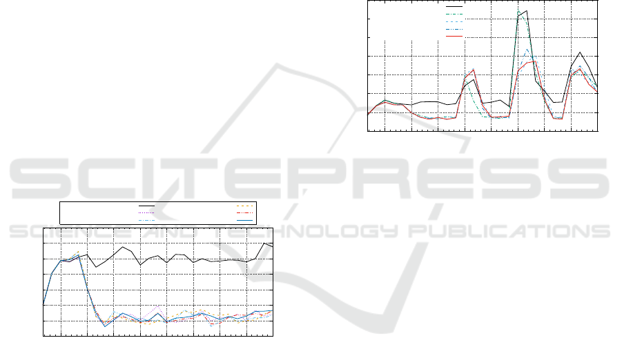
Fig. 4 indicates that OTC with and without routing is

able to drastically reduce the overall delay compared

to ﬁxed-time signalisation. The ﬁgure shows the av-

erage travel time in seconds per kilometre for a simu-

lated scenario of 2 hours. The compliance rate was set

to 70%. The mean delay is given in brackets behind

the protocol’s name.

130

140

150

160

170

180

190

200

00:15 00:30 00:45 01:00 01:15 01:30 01:45 02:00 02:15

Travel time (s/km)

Time (min.)

Fixed-time (180.20 s)

OTC (148.64 s)

LSR (148.14 s)

Temporal LSR (148.64 s)

DVR (148.20 s)

Temporal DVR (148.76 s)

Figure 4: Travel times for the regular Manhattan scenario.

The ﬁrst 15 minutes of the simulation represent

the warm-up time, where OTC gathers data to cali-

brate the forecast methods. Each observer/controller

needs to populate its initial empty database of map-

pings between optimised signal plans and monitored

trafﬁc demands. Therefore, the overall performance

is identical. Afterwards, it can be seen that the static

ﬁxed-time signal plans are not able to reduce the neg-

ative impacts of the trafﬁc demands. Table 1 presents

the average travel times over all trips, the average fuel

consumption and the average CO

emissions per ve-

hicle for the reference run and the proactive routing

protocols with different compliance rates. Reductions

compared to the reference run are given in brackets.

Not only is the travel time reduced signiﬁcantly (17%)

in comparison to the reference run, but so are the fuel

consumption (4% to 6%) and the pollution emissions

(2% to 3.3%). These results must be interpreted with

caution. During undisturbed conditions, an improved

signalisation alone is enough to guarantee a reduction

of queues. OTC without routing already reduces the

travel time to 227.6 seconds.

In contrast to the undisturbed scenario, the con-

gested scenario clearly shows the beneﬁt of DRG dur-

ing incidents. Table 2 summarises the evaluation re-

sults. The routing mechanism gives drivers indica-

tions how to avoid congested areas. It reduces the

average travel time by 10% (TLSR) to 11% (TDVR)

(Fig. 5) for a compliance rate of 70%.

100

150

200

250

300

350

400

450

00:15 00:30 00:45 01:00 01:15 01:30 01:45 02:00 02:15

Travel time (s/km)

Time (min.)

Fixed-time (216.6 s)

LSR (194.4 s)

Temporal LSR (192.1 s)

DVR (191.3 s)

Temporal DVR (189.4 s)

Figure 5: Travel times for the congested scenario.

The best performance was delivered by TDVR

achieving the highest travel time reduction. At 1:45,

during a severe incident, TDVR reduces the average

travel time to 282 seconds per kilometre (33% im-

provement over the reference run with 421 seconds

and 30% improvement over OTC without routing with

408 seconds). This indicates that TDVR correctly

forecasted the upcoming congestion due to the inci-

dent, preventing more severe disturbances. This re-

sembles an improvement of 4.0% compared to OTC

without routing with an average trip travel time of 320

seconds. The decrease in travel time is achieved by

re-routing drivers over alternative routes, which can

be longer than the planned one. Therefore, the use of

routing protocols sometimes leads to slightly higher

fuel consumption and CO

emissions.

Fig. 6 and Fig. 7 present the average travel times

evaluated for several compliance rates. A higher com-

pliance rate means that drivers are more likely to fol-

low the given routing proposals. The ﬁgure’s horizon-

tal axis shows the simulation time and the vertical axis

shows the average travel time in seconds per kilome-

tre. Our results suggest that the beneﬁt of all routing

protocols increases for higher compliance rates.

VEHITS 2016 - International Conference on Vehicle Technology and Intelligent Transport Systems

184

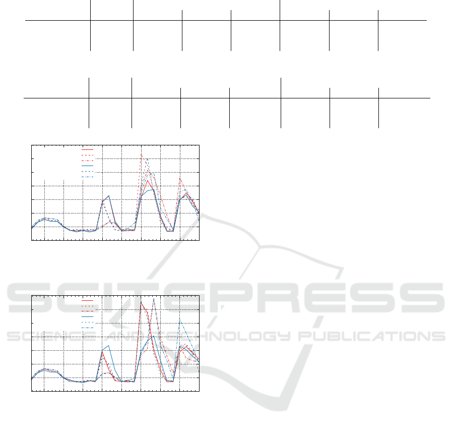
Table 1: Results for the regular scenario with TDVR and TLSR.

Fixed-time TDVR TLSR

0.7 0.4 0.1 0.7 0.4 0.1

Travel time [s/veh] 275 228 (17.1%) 228 (17.1%) 228 (17.1%) 227 (17.5%) 230 (16.4%) 227 (17.5%)

Fuel [l/100km] 15.1 14.5 (4.0%) 14.4 (4.6%) 14.2 (5.8%) 14.5 (4.0%) 14.6 (3.4%) 14.2 (5.8%)

[g/veh] 518.5 506.0 (2.4%) 504.7 (2.6%) 501.4 (3.3%) 504.7 (2.7%) 508.3 (2.0%) 501.6 (3.3%)

Table 2: Results for the congested scenario with TDVR and TLSR.

Fixed-time TDVR TLSR

0.7 0.4 0.1 0.7 0.4 0.1

Travel time [s/veh] 345 306 (11.3%) 310 (10.1%) 320 (7.2%) 310 (10.1%) 313 (9.2%) 335 (2.9%)

Fuel [l/100km] 16.6 16.4 (1.2%) 16.3 (1.8%) 16.6 (0.0%) 16.6 (0.0%) 16.4 (1.2%) 17.0 (-2.4%)

[g/veh] 549.6 543.6 (1.1%) 545.7 (0.7%) 551.8 (-0.4%) 547.2 (0.4%) 547.0 (0.5%) 562.3 (-2.3%)

100

150

200

250

300

350

400

450

00:15 00:30 00:45 01:00 01:15 01:30 01:45 02:00 02:15

Travel time (s/km)

Time (min.)

DVR 0.7 (191.31 s)

DVR 0.4 (193.73 s)

DVR 0.1 (200.47 s)

TDVR 0.7 (189.44 s)

TDVR 0.4 (190.32 s)

TDVR 0.1 (195.33 s)

Figure 6: Compliance rates for the congested Manhattan

scenario with DVR.

100

150

200

250

300

350

400

450

00:15 00:30 00:45 01:00 01:15 01:30 01:45 02:00 02:15

Travel time (s/km)

Time (min.)

LSR 0.7 (194.39 s)

LSR 0.4 (194.54 s)

LSR 0.1 (194.75 s)

TLSR 0.7 (192.13 s)

TLSR 0.4 (192.55 s)

TLSR 0.1 (205.29 s)

Figure 7: Compliance rates for the congested Manhattan

scenario with LSR.

5.2.2 Regional Scenario

Table 3 depicts the comparison of communicational

and computational effort between regional protocols

and the basic variants. The table shows the number

of messages each TLC has to send during one iter-

ation of the executed routing protocol and the aver-

age runtime in seconds of a complete protocol run.

The results clearly depict that the regional protocols

decrease the number of messages and the computa-

tional overhead. The reference run has no communi-

cation between TLCs and therefore no sent messages.

The anticipatory protocols need more computational

power to compute the forecasts for all sections and

turnings of the network, leading to longer runtime.

As Table 4 indicates, the regional protocols do not

or only to a slight extend increase the average travel

time. The simpliﬁcation of the communication due to

the regional aggregation of RCs offers equally good

route recommendations while reducing the communi-

cation and computational effort.

6 CONCLUSION

This paper presented two novel time-aware, antici-

patory routing protocols (TLSR and TDVR) for dy-

namic, proactive trafﬁc guidance in urban road net-

works. The well-known Internet protocols Distance

Vector Routing and Link State Routing have been

extended, utilising trafﬁc ﬂow forecasts to compute

the best routes through a road network. The routes

are determined by a self-organised approach, extend-

ing parametrisable trafﬁc light controllers. The route

recommendations are visualised by Variable Message

Signs at each intersection, guiding drivers from inter-

section to intersection on a next-hop basis. The pro-

tocols were evaluated with compliance rates of 10%,

40% and 70%. A simulation study investigated the

beneﬁts of these protocols under disturbed and undis-

turbed conditions in two different networks. Our ﬁnd-

ings strongly support the view that the consideration

of trafﬁc ﬂow forecasts leads to a decrease in system-

wide travel times for urban vehicular trafﬁc. Conse-

quently, this leads to a reduction in pollution emis-

sions and fuel consumption. In general, this counts

especially for disturbed and congested conditions, but

to a limited extend also for medium and low trafﬁc

saturations. The beneﬁt increases for higher compli-

ance rates. During undisturbed conditions, an im-

proved signalisation alone is enough to guarantee a

reduction of queues. The dynamic route guidance im-

proves the network’s robustness by guiding road users

on alternative routes around blocked areas. The Tem-

poral Distance Vector Routing protocol showed to be

the most beneﬁcial approach, not only for congested

Forecast-augmented Route Guidance in Urban Trafﬁc Networks based on Infrastructure Observations

185

Table 3: Comparison of regional and basic protocols in terms of sent messages and computational time.

Fixed-time DVR Reg. DVR TDVR Reg. TDVR LSR Reg. LSR TLSR Reg. TLSR

Messages (#/RC/iter.) 0 1437 133 1463 133 35 25 35 24

Runtime (s) 10 360 105 1400 400 280 270 330 370

Table 4: Travel time of regional and basic protocols for the regional scenario.

DVR Reg. DVR TDVR Reg. TDVR LSR Reg. LSR TLSR Reg. TLSR

Undisturbed: Travel time [s/veh] 119.83 119.27 119.49 119.30 119.73 119.76 119.39 121.68

Disturbed: Travel time [s/veh] 127.83 128.44 128.41 127.15 128.69 129.14 129.00 130.18

but also during free ﬂow conditions. The communi-

cational overhead and the computational costs can be

reduced by partitioning a larger network into smaller

sub-networks via the Border-Gateway-Protocol.

REFERENCES

Barcelo, J. and Casas, J. (2002). Dynamic network simu-

lation with AIMSUN. In Proc. of the Int. Symp. on

Transp. Simul., pages 1–25. Kluwer.

Claes, R., Holvoet, T., and Weyns, D. (2011). A decen-

tralized approach for anticipatory vehicle routing us-

ing delegate multiagent systems. IEEE Trans. on Int.

Transp. Systems, 12:364–373.

Dijkstra, E. W. (1959). A note on two problems in connex-

ion with graphs. Numerische Mathematik, 1(1):269–

271.

Dong, J., Mahmassani, H., and Lu, C.-C. (2006). How reli-

able is this route: Predictive travel time and reliability

for anticipatory traveler information systems. Journal

of the Transp. Research Board, (1980):117–125.

Dong, W. (2011). An overview of in-vehicle route guidance

system. 34th Australasian Transp. Research Forum

(ATRF 2011), Adelaide, Australia, 28-30 Sept. 2011.

Emmerink, R. H. M., Nijkamp, P., and Rietveld, P. (1996).

Variable message signs and radio trafﬁc informa-

tion, an integrated empirical analysis of drivers route

choice behaviour. In Transp. Research Part A: Policy

and Practice, volume 30, pages 135–153.

Erke, A., Sagberg, F., and Hagman, R. (2007). Effects of

route guidance variable message signs (vms) on driver

behaviour. Transp. Research Part F: Trafﬁc Psychol-

ogy and Behaviour, 10(6):447 – 457.

F.S. Zuurbier, J. v. L. and van Zuylen, H. (2006). Com-

parison study of decentralized feedback strategies for

route guidance purposes. In Proc. of the 9th TRAIL

Congress, pages 1–15.

Fu, L. (2001). An adaptive routing algorithm for in-vehicle

route guidance systems with real-time information.

Transp. Research Part B, 35(8):749–765.

Hart, P. E., Nilsson, N. J., and Raphael, B. (1968). A formal

basis for the heuristic determination of minimum cost

paths. IEEE Trans. on Systems Science and Cybernet-

ics, 4(2):100–107.

Horst F. Wedde et al. (2007). Highly Dynamic and Adap-

tive Trafﬁc Congestion Avoidance in Real-Time In-

spired by Honey Bee Behavior. In Mobilit

at und

Echtzeit – Fachtagung der GI-Fachgruppe Echtzeit-

systeme, pages 21–31. Springer.

Hyndman, R. J. and Koehler, A. B. (2006). Another look at

measures of forecast accuracy. International Journal

of Forecasting, pages 679–688.

Kaplan, E. (2005). Understanding GPS - Principles and

applications. Artech House, 2nd edition edition.

Nannicini, G., Delling, D., Schultes, D., and Liberti, L.

(2012). Bidirectional a* search on time-dependent

road networks. Netw., 59(2):240–251.

Panis, L. I., Broekx, S., and Liu, R. (2006). Modelling in-

stantaneous trafﬁc emission and the inﬂuence of traf-

ﬁc speed limits. Science of The Total Environment,

371(13):270 – 285.

Parkany, E. and Xie, P. C. (2005). A complete review of in-

cident detection algorithms & their deployment: What

works and what doesn’t. Technical report, Fall River,

MA: New England Transp. Consortium.

Prothmann, H., Tomforde, S., Branke, J., H

ahner, J.,

uller-Schloer, C., and Schmeck, H. (2011). Organic

Trafﬁc Control. In Organic Computing – A Paradigm

Shift for Complex Systems, chapter 5.1, pages 431–

446. Birkh

auser.

Prothmann, H., Tomforde, S., Lyda, J., Branke, J., H

ahner,

J., M

uller-Schloer, C., and Schmeck, H. (2012). Self-

organised routing for road networks. In Proc. of the

6. Int. Workshop on Self-Organizing Systems, LNCS

7166, pages 48–59. Springer.

Schmitt, E. J. and Jula, H. (2006). Vehicle route guidance

systems: classiﬁcation and comparison. 2006 IEEE

Intelligent Transp. Systems Conference, 1:242–247.

Sommer, M., Tomforde, S., H

ahner, J., and Auer, D. (2015).

Learning a dynamic re-combination strategy of fore-

cast techniques at runtime. In Proc. of IEEE Int. Conf.

on Autonomic Computing (ICAC), pages 261–266.

Tanenbaum, A. S. (2002). Computer Networks. Pearson,

4th edition.

Tomforde, S., Prothmann, H., Branke, J., H

ahner, J.,

uller-Schloer, C., and Schmeck, H. (2010). Pos-

sibilities and limitations of decentralised trafﬁc con-

trol systems. In IEEE World Congress on Comp. Int.,

pages 3298–3306. IEEE.

Webster, F. V. (1958). Trafﬁc signal settings. Road Research

Technical Paper No. 39, Road Research Laboratory,

England, HMSO.

Wunderlich, K. E., Kaufman, D. E., and Smith, R. L.

(2000). Link travel time prediction for decentralized

route guidance architectures. IEEE Transactions on

Intelligent Transp. Systems, 1(1):4–14.

VEHITS 2016 - International Conference on Vehicle Technology and Intelligent Transport Systems

186