
Incorporating Explanatory Effects of Neighbour Airports in
Forecasting Models for Airline Passenger Volumes
Nilgun Ferhatosmanoglu
1
and Betul Macit
2
1
Department of Industrial and Systems Engineering, University of Turkish Aeronautical Association, Ankara, Turkey
2
Department of Industrial Engineering, Gazi University, Ankara, Turkey
Keywords: Forecasting, Airport Networks, TBATS, Regression with ARIMA Errors, Airline Passenger Volumes,
Neighbour Effects in Modelling.
Abstract: Forecasting airline passenger volumes can be helpful for flight and airport capacity planning. While there
are many parameters affecting the passenger volume, to our knowledge no work has directly studied the
effect of neighbour airports in modelling of passenger volumes. We develop an integrated model for
forecasting the number of passengers arriving/departing an airport, considering the airport’s interactions
with its neighbour airports. In particular, we analyse the time series of the flights arriving to and departing
from two largest airports in Turkey, namely Ankara Esenboga and Istanbul Ataturk Airports, and explore
the interactions between these airports by using them as regressors for each other. We also apply
independent models based on TBATS which was previously proposed in the literature to handle multiple
seasonalities. In our experiments, TBATS performs better than ARIMA for independent modelling, and
TBATS with multiple seasonal periods outperforms TBATS with single seasonality in majority of the cases.
In several cases, the forecasting accuracy increases when the neighbour airports’ traffic data is used in
modeling the passenger volumes.
1 INTRODUCTION
Civil aviation authorities and airline companies need
short and long term forecasts for effective flight and
capacity planning. A wide range of forecasting
models are developed including econometric
modelling, univariate time series modelling, time
series decomposition, non-linear regression models
and gravity models (Scarpel, 2013). While it is
intuitive that the traffic of an airport is not
independent of its neighbour airports, to our
knowledge this is not directly taken into
consideration in modelling and forecasting airport
traffic. Research is needed to investigate how the
traffic model of an airport can incorporate its
‘neighbours’ traffic as they affect each other
possibly with a small time shift. In this paper, we
consider interactions between neighbour airports in
developing time series forecasting models for air
traffic volumes. We handle two neighbour airports
as a dyad in an airport network and compare
independent and neighbour-dependent models to
forecast the number of passengers for particular
routes.
As a case study, we analyse time series patterns
of domestic and international flights arriving to and
departing from Ataturk and Esenboga International
Airports in Turkey over the course of a year. We
propose a neighbour-dependent approach using
regression with ARIMA errors and explore
explanatory relations by regressor time series. For
independent modelling, we consider ARIMA and
TBATS models for developing independent
forecasting models. TBATS (Trigonometric, Box-
Cox transform, ARMA errors, Trend, and Seasonal
components) model was proposed to deal over
parameterization and handle both non-integer period
and dual-calendar effects (De Livera et al., 2011).
ARIMA models enable fitting the patterns in data
with smallest number of estimated parameters.
TBATS handles multiple seasonality which we
observe in Turkish flight data. We elaborate
accuracy performance of TBATS method and
ARIMA models in independent modelling as well.
By comparing the accuracy of independent and
dependent models we are able to explore
contribution of neighbour relations on forecasting
performance.
178
Ferhatosmanoglu, N. and Macit, B.
Incorporating Explanatory Effects of Neighbour Airports in Forecasting Models for Airline Passenger Volumes.
DOI: 10.5220/0005752801780185
In Proceedings of 5th the International Conference on Operations Research and Enterprise Systems (ICORES 2016), pages 178-185
ISBN: 978-989-758-171-7
Copyright
c
2016 by SCITEPRESS – Science and Technology Publications, Lda. All rights reserved

In our experiments, TBATS performs better than
ARIMA for independent modelling. TBATS models
with multiple seasonal periods perform better than
models with single seasonality. These results verify
that TBATS model performs well in airline data
with multiple seasonality. Using explanatory time
series of neighbours’ air passenger volumes is found
to be useful in several cases.
The remainder of the paper contains the
following sections. First, we present a literature
overview on air passenger flow problem and the
forecasting methods used in this study. We then
present the proposed methodology and empirical
results. Finally, we conclude with future research
directions.
2 RELATED WORK
Air transportation has achieved a remarkable growth
both worldwide and in Turkey, e.g., the total number
of passengers in Turkey has risen 14.3% in the last
decade (TOBB, 2013). According to
EUROCONTROL forecasts, Turkey will be the
arrival or departure point for the greatest number of
extra flights in the future European airspace by 2035
(EUROCONTROL, 2013). In our study, we generate
forecasting models for the number of air travel
passengers for different routes between Ankara
Esenboga and Istanbul Ataturk Airports.
Several methods have been proposed for
forecasting the number of air travel passengers in the
context of air travel demand, pax growth and air
travel flow. Traditional methods, such as neural
networks, exponential smoothing, Box-Jenkins, and
Holt-Winters, are commonly applied in this context.
Nam et al. use neural networks for predicting
international air passenger volume between US and
Mexico and compare them with regression and
exponential smoothing forecasting models (Nam et
al., 1997). Neural network models are also compared
with well-known Box-Jenkins and Holt-Winters
Methods (Faraway et al., 1998). In an application
study, neural networks are shown to outperform the
traditional econometric approach for forecasting
Brazilian air transport passenger traffic (Alekseev et
al., 2009).
Samagaio and Wolters propose ARIMA and
exponential smoothing models for forecasting the
number of passengers for 2008-2020 to help
decision making for establishing a new airport
(Samagaio et al., 2010). An application of fuzzy
regression model is developed to forecast the
demand of Rhodes airport (Profillidis, 2000).
Grosche et al. propose two gravity models using
geo-economic factors as independent variables for
estimation of airline passenger volume between city
pairs (Grosche et al., 2007). Fildes et al. explore the
relations between air traffic flows to different
countries by pooled ADL model (Flides et al., 2011).
They enhance their models with “world trade”
variable and conclude that pooled ADL model with
“world trade” variable outperformed the alternatives.
Benitez et al. propose a modified Grey Model for
airlines routes pax growth for long lead-time
(Benitez et al., 2013). ARIMAX and SARIMA
based models are recently used to forecast Hong
Kong airport's passenger throughput till 2015 (Tsui
et al., 2014). Time series involved in our analysis
involve multiple seasonal patterns. Hence we use a
recent proposal, TBATS, which handles multiple
seasonality (De Livera et al., 2011).
3 METHODOLOGY
In this section, we highlight the methods for
handling the seasonality from the literature and
introduce the details of our methodology to
incorporate the interactions of two airports into their
forecasting models. In particular, we study Ataturk
and Esenboga Airports in Turkey and investigate if
they affect each other while forecasting their
passenger volumes. The data set of the number of
passengers for Ataturk and Esenboga Airports in
2011 is obtained from the General Directorate of
State Airports Authority of Turkey. Eight time series
of the number of passengers in international and
domestic incoming & outgoing flights of these
airports are generated. We build models both
independently and neighbour-dependently and
compare their performance. For independent models,
which do not consider the neighbour effects, we
investigate the conventional ARIMA and the
recently proposed TBATS approach on forecasting
airline passenger volumes. We also study a
neighbour dependent approach where we use the
traditional regression with ARIMA errors approach
and incorporate the neighbour effects as a regressor
time series.
We now summarize the methods we applied in
our independent modelling and present our
neighbour dependent modelling approach.
Incorporating Explanatory Effects of Neighbour Airports in Forecasting Models for Airline Passenger Volumes
179

3.1 Independent Modelling with
ARIMA and TBATS
We apply ARIMA and TBATS methods for
independent modelling and analysis. ARIMA (Auto-
Regressive Integrated Moving Average) is a basic
approach for analysis and forecasting of equally
spaced univariate time series data. Box and Jenkins
proposed an entire family of ARIMA models and an
analysis to find the smallest number of estimated
parameters needed to fit the patterns in the data.
Box-Jenkins methodology involves three steps;
identification, estimation and diagnostic checking
(Pankratz, 1983). As a baseline for comparison, we
use automated ARIMA model fitting function in
forecast package of R programming.
Our preliminary data analysis reveals that our
passenger volume time series involve multiple
seasonality. Most commonly used methods for
modelling seasonal time series, such as Holt-
Winters, exponential smoothing approach, ARIMA
models, suffer dealing with double seasonality.
Recently, exponentially weighted methods for
multiple seasonal time series are proposed (De
Livera, 2010). To deal with double seasonality, an
extension of Holt-Winter is proposed (Taylor, 2003).
In another study, a multiple seasonal method is
developed that allows the seasonal cycle to be
updated more than once during the period of the
cycle (Gould et al, 2007). Also time series may have
complex seasonal patterns such as patterns with a
non-integer period, have high frequency multiple
seasonal patterns or may have dual calendar effects.
De Livera et al. propose a new innovations state
space model based approach that is capable of
dealing over parameterization and tackling with both
non-integer period and dual-calendar effects (De
Livera et al., 2011). They improve the traditional
single seasonal exponential smoothing methods, and
introduce two algorithms. They propose TBATS,
which stands for Trigonometric, Box-Cox transform,
ARMA errors, Trend, and Seasonal components
Model.
The Box-Cox transformation, ARMA errors,
Trend and Seasonal components (BATS) are defined
by;
()
=
(
−1)/ℎ ≠ 0
ℎ = 0
,
()
=
+
+
∑
+
(3.1)
=
+
+
(3.2)
=
(
1−
)
+
+
(3.3)
()
=
()
+
Υ
(3.4)
where ∈ is the Box-Cox transformation
parameter,
……
denote the constant periods
of the n seasonal components, is the long run
trend,
is an (,) process with Gaussian
white noise innovations having zero mean and
constant variance, and for =1,…., ,
is the
local stochastic level,
is the short term trend and
()
is the stochastic level of the −ℎ seasonal
component.
De Livera et al. proposed a new trigonometric
representation of seasonal components based on
Fourier series.
()
=
∑
,
()
(3.5)
,
()
=
,
()
()
+
,
∗()
()
+
Υ
()
(3.6)
,
∗()
=−
,
(
)
+
,
∗
(
)
(
)
+
Υ
()
(3.7)
Where Υ
()
and Υ
()
are smoothing parameters,
()
=2/
.
,
()
describe the stochastic level of
the i
th
seasonal component, and the stochastic
growth in the level of the i
th
component that is
needed to describe the change in the seasonal
component over time is described by
,
∗()
. The
number of harmonics required for the i
th
seasonal
component is denoted by
(De Livera et al.,
2011). The performance of these approaches on
forecasting passenger volumes is presented in the
experimental section.
3.2 Neighbour Dependent Modelling
In neighbour-dependent analysis, we incorporate the
explanatory effects of regressor time series of
neighbour airports using regression with ARIMA
errors method.
=
+
,
+⋯+
,
+
(3.8)
One of the key assumptions of multiple
regression is that
is an uncorrelated series. For
regression with ARIMA, it is considered that
contains autocorrelations. The resulting model is
now a regression model with ARIMA errors.
Equation 3.8 still holds but
is modeled as an
ARIMA process. We follow the notations of
Makridakis et al. (1998) for stating regression with
ARIMA model. For example, if
is an ARIMA (1,
1, 1) model, 3.8 can be written
=
+
,
+⋯+
,
+
(3.9)
ICORES 2016 - 5th International Conference on Operations Research and Enterprise Systems
180
where
(
1−
)(
1−
)
=
(
1−
)
and
is a white-noise series.
For identification of regressor time series, we
analyse the cross correlation between time series and
consider highly correlated and weakly correlated
series for building significant explanatory relations.
Initially we build regression with ARIMA models in
line with the correlation between Ataturk and
Esenboga series and we add regressor variables into
the model individually. Then we check the internal
cross correlation in Ataturk and Esenboga series in
order to identify regressor pairs. In this analysis it is
revealed that all series in Ataturk dataset are highly
correlated, hence we do not use any pairs while
building explanatory models for Esenboga series
with Ataturk data. In Esenboga dataset, we find out
that Esenboga International Incoming Passengers
data is weakly correlated with the rest of the series
and this result enables us to use pairs as regressors
while building explanatory models for Ataturk data.
4 EMPIRICAL ANALYSIS
To evaluate the performance of the presented
methods for forecasting the number of passengers
for an airport, we collected a list of real time series
as presented in Table 1. We adjusted our dataset by
forming equal time intervals for all time series.
Volumes of passengers are quarterly aggregated by
six-hour time periods for each day that helps to
detect seasonal patterns inherent in data. Following
the data adjustment, we divided the available one-
year data into training and test sets. We built models
with a training set involving 1092 data points and
tested the models with 124 data points.
Table 1: List of analysed time series.
Ataturk A. Domestic Flights Incoming Number
of Passengers (ADI)
Ataturk A. Domestic Flights Outgoing Number
of Passengers (ADO)
Ataturk A. International Flights Incoming
Number of Passengers (AII)
Ataturk A. International Flights Outgoing
Number of Passengers (AIO)
Esenboga A. Domestic Flights Incoming
Number of Passengers (EDI)
Esenboga A. Domestic Flights Outgoing
Number of Passengers (EDO)
Esenboga A. International Flights Incoming
Number of Passengers (EII)
Esenboga A. International Flights Outgoing
Number of Passengers (EIO)
All series have multiple seasonal patterns and
high frequency seasonality. For each set of data, four
independent models are fit: (I) ARIMA model with
frequency=4,(II) ARIMA model with frequency=28,
(III) TBATS Model with frequency=28 and (IV)
TBATS Model with double seasonality. For
neighbour-dependent analysis, we build regression
with ARIMA models with convenient regressor time
series. MAPE (Mean Absolute Percentage Error) is
the preferred forecasting accuracy measure for
simplicity when all data are positive and much
greater than zero (Hyndman and Koehler, 2006). We
also report MAE (Mean Absolute Percentage Error)
and MASE (Mean Absolute Scaled Error) based
results of our experiments (Hyndman and Koehler,
2006).
4.1 Independent Analysis with ARIMA
and TBATS Models
We first analyse the time-series, ACF
(Autocorrelation Function) and PACF (Partial
Autocorrelation Function) plots for all data sets. For
brevity, we present the models for one representative
data set (i.e., ADI) in detail and for the rest of the
series we present the model results.
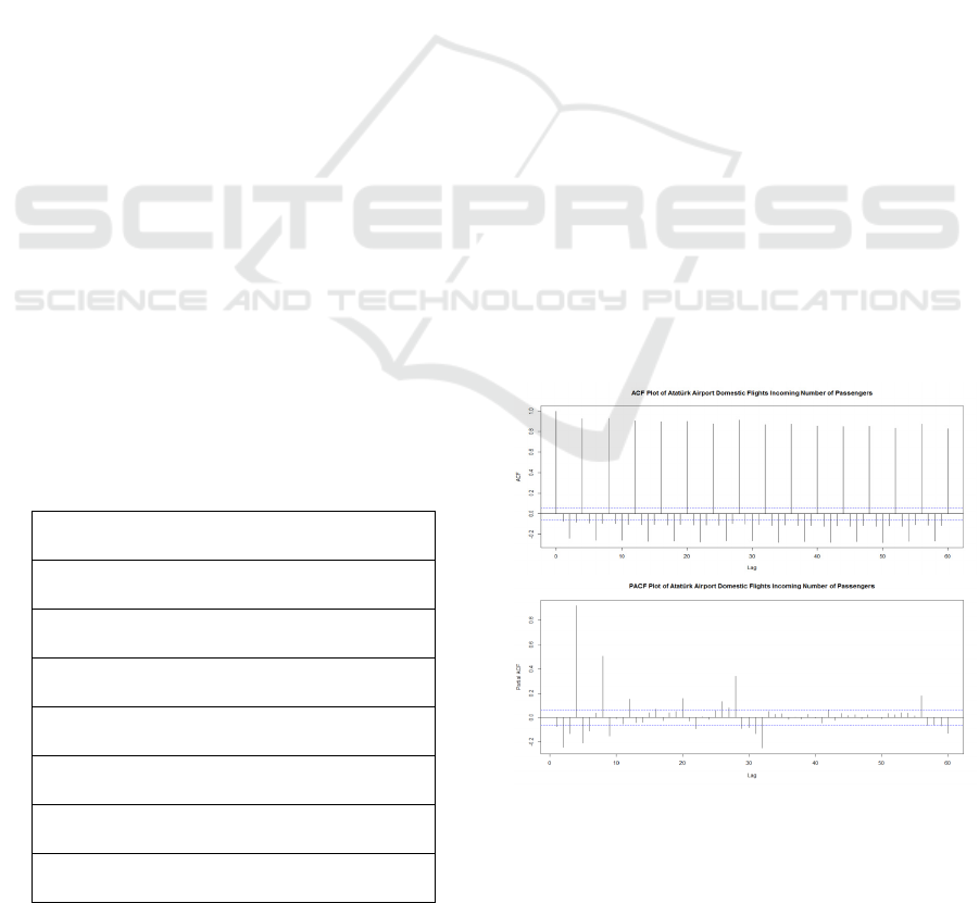
The ACF and PACF plots illustrate two seasonal
periods (Figure 1). The first seasonality arises from
aggregating daily data quarterly by 6 hour time
periods and the seasonal period is four. The second
seasonality is observed with the help of PACF plot,
28 periods indicates the weekly seasonality in the
training data set.
Figure 1: ACF and PACF plots of ADI data.
Based on these results, we fit four independent
models. (I) ARIMA model with frequency=4, (II)
Incorporating Explanatory Effects of Neighbour Airports in Forecasting Models for Airline Passenger Volumes
181
ARIMA model with frequency=28, (III) TBATS
Model with frequency=28 and (IV) TBATS Model
with double seasonality for each dataset. We
developed these four independent models for each of
the eight time series and according to MAPE (Mean
Absolute Percentage Error) measure we present the
best independent models for each of the time series
in Table 3.
Table 2: Forecasting Accuracy of Independent Models for
ADI.
Model MAE MAPE MASE
ARIMA(0,1,2)(2,0,0)[4] 727.15 19.81 1.24
ARIMA(4,0,0)(0,1,1)[28] 513.41 12.45 1.05
TBATS(0.71, {2,1},
0.809, {<28,7>})
455.22 11.69 0.93
TBATS(0.684, {2,1},
0.861, {<4,1>, <28,6>})
441.30 11.07 0.90
Table 3: Best Independent Models for All Time Series.
Data The Best Model MAPE
ADO TBATS(1, {2,1}, -, {<28,8>}) 12.03
AII ARIMA(4,0,0)(0,1,1)[28] 9.24
AIO
TBATS(0.998, {5,4}, -, {<4,1>,
<28,5>})
9.70
EDI
TBATS(0.999, {4,5}, -,
{<28,8>})
11.94
EDO ARIMA(4,0,0)(0,1,1)[28] 7.85
EII
TBATS(0.327, {4,4}, -,
{<28,7>})
52.02
EIO
TBATS(0.095, {0,0}, -, {<4,1>,
<28,5>})
56.58
In half of the independent models, TBATS
model with multiple seasonality outperformed other
models according to MAPE measure. In the second
half of the independent models, TBATS and
ARIMA models with weekly seasonality outperform
other models. These results show that TBATS
successfully handles multiple seasonality in our
airline passenger volume time series, and it yields
better forecasting accuracies than the traditional
ARIMA approach.
4.2 Neighbour-dependent Analysis with
Regression with ARIMA Errors
We generated a cross correlation matrix for time
series in the preliminary analysis phase. Table 4
depicts the cross correlation in all series. According
to correlation values in this matrix, we establish the
explanatory relations between time series and we
build regression with ARIMA models with regressor
time series. While building regression with ARIMA
models for Ataturk Airport time series data, initially
we analysed cross correlation with Esenboga Airport
data. For example, ADI data can be paired with data
of EIO, EDI and EDO data as explanatory Regressor
variables.
Table 4: Cross Correlation between All Series.
ADI ADO AII AIO EDI EDO EII EIO
ADI 1.00 0.53 0.44 0.88 0.72 0.87 0.16 0.57
ADO 0.53 1.00 0.83 0.50 0.53 0.55 0.51 0.40
AII 0.44 0.83 1.00 0.46 0.42 0.39 0.62 0.31
AIO 0.88 0.50 0.46 1.00 0.64 0.79 0.21 0.59
EDI 0.72 0.53 0.42 0.64 1.00 0.74 0.26 0.34
EDO 0.87 0.55 0.39 0.79 0.74 1.00 0.20 0.53
EII 0.16 0.51 0.62 0.21 0.26 0.20 1.00 0.27
EIO 0.57 0.40 0.31 0.59 0.34 0.53 0.27 1.00
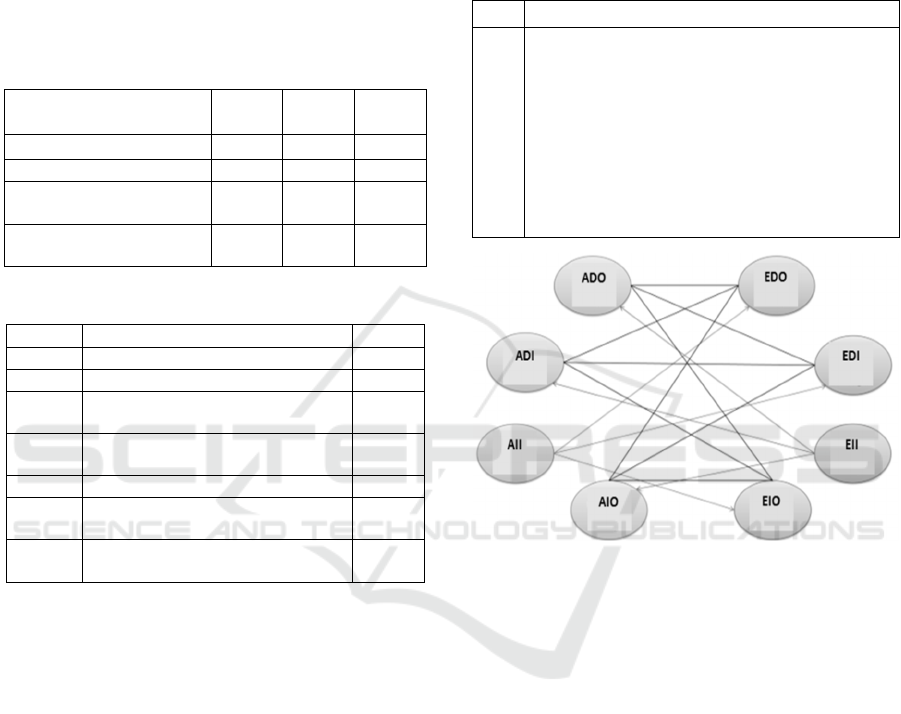
Figure 2: Explanatory Relations between Time Series.
Taking into account all possible routes and
connections we consider the explanatory relations in
Figure 2. In this figure, black undirected edges
represent the mutual interactions, the gray directed
edges represent the single sided influence.
According to these relations, it is clear that the
volume of passengers in international incoming
flights cannot be explained by neighbour effects.
This observation also makes sense in practice.
Hence we do not build regression with ARIMA
models for international incoming passengers data.
But we consider these series as explanatory variables
in other models.
When we consider all possible routes and
connections that may affect ADI data, we may
expect ADI data to be correlated with all series in
Esenboga data. We build seven neighbour-
dependent models for ADI dataset and compare
contribution of regression variables in forecasting
performance. Regression with ARIMA models for
ADI data is presented in Table 5. We find out that
ICORES 2016 - 5th International Conference on Operations Research and Enterprise Systems
182

the best model in neighbour-dependent models is
regression with ARIMA model including EDO data
as regressor variable, and it performs better than an
independent ARIMA model (seasonal period: 4). We
compare these neighbour dependent model results
with the independent model results in Table 6 by
MAPE accuracy measure. For this data set, the best
model out of all models is the independent TBATS
model with multiple seasonality.
Table 5: Regression with ARIMA models for ADI Data
(Neighbour dependent models).
Model MAE MAPE MASE
ARIMA(0,1,2)(2,0,0)[4]
REG. with EDI
721.32 18.80 1.23
ARIMA(0,1,3)(2,0,0)[4]
REG. with EDO
632.39 16.36 1.08
ARIMA(1,1,1)(2,0,0)[4]
REG. with EII
1063.30 32.13 1.82
ARIMA(3,1,1)(0,0,1)[4]
REG. with EIO
778.20 21.99 1.33
ARIMA(0,1,3)(2,0,0)[4]
REG. with EII and EIO
1020.09 30.04 1.74
ARIMA(1,1,1)(2,0,0)[4]
REG. with EII and EDI
690.17 17.71 1.18
ARIMA(0,1,3)(2,0,0)[4]
REG. with EII and EDO
619.53 15.88 1.06
Table 6: Forecasting Accuracy of Independent Models for
ADI.
Model MAE MAPE MASE
ARIMA(0,1,2)(2,0,0)[4] 727.15 19.81 1.24
ARIMA(4,0,0)(0,1,1)[28] 513.41 12.45 1.05
TBATS(0.71, {2,1},
0.809, {<28,7>})
455.22 11.69 0.93
TBATS(0.684, {2,1},
0.861, {<4,1>, <28,6>})
441.30 11.07 0.90
Ataturk Airport Domestic and International
Outgoing Passengers data are correlated with all
series in Esenboga data. For this reason, we add all
series as regressor variables individually and we also
consider the weakly interrelated Esenboga time
series pairs as regressor variables. Regression with
ARIMA models with the best test results are
presented in Table 7.
The best model for ADO data in the neighbour-
dependent approach is when EDI is used as a
regressor variable. It outperforms the worst model,
ARIMA (seasonal period: 4) in independent models.
For ADO data, the best model out of all models is
the independent TBATS model with single
seasonality. The comparison of the best performing
dependent and independent models is presented in
Table 8.
For AIO data, the best neighbour-dependent
model is the regression with ARIMA model
including EDO data. The best model out of all
models is the independent TBATS model with
multiple seasonality. The comparison of the best
performing dependent and independent models is
presented in Table 9.
Table 7: The Best Regression with ARIMA models for
ADO and AIO Data.
Data The Best Neighbour
Dependent Models
MAPE
ADO
ARIMA(3,1,0)(0,0,1)[4]
REG. with EDI
16.59
AIO
ARIMA(0,1,1)(2,0,1)[4
REG. with EDI
11.48
Table 8: Comparison of Models for ADO Data.
Data Models MAPE
ADO
ARIMA(3,1,0)(0,0,1)[4]
REG. with EDI
16.59
TBATS(1, {2,1}, -, {<28,8>}) 12.03
In regression with ARIMA models for Esenboga
Airport, due to the strong cross correlation in
Ataturk Airport time series data, each regression
with ARIMA model built for Esenboga Airport
routes involves one of the Ataturk Airport time
series. The accuracy performance of regression with
ARIMA models is demonstrated in Tables 10-11.
Table 9: Comparison of Neighbour Dependent and
Independent Models for AIO Data.
Data Models MAPE
AIO
ARIMA(0,1,1)(2,0,1)[4] REG.
with EDI
11.48
TBATS(0.998, {5,4}, -,
{
<4,1>, <28,5>
}
)
9.70
Table 10: Regression with ARIMA models for EDI Data
(Neighbour Dependent Models).
Model MAE MAPE MASE
ARIMA(3,1,1)(0,0,1)[4]
REG.with ADI
257.95 12.12 0.70
ARIMA(3,1,0)(2,0,0)[4]
REG.with ADO
372.63 15.94 1.02
ARIMA(0,1,3)(1,0,1)[4]
with drift REG. with AII
254.69 12.93 0.70
ARIMA(0,1,3)(1,0,1)[4]
with drift REG. with
AIO
277.25 14.20 0.76
Incorporating Explanatory Effects of Neighbour Airports in Forecasting Models for Airline Passenger Volumes
183

For EDI data, the best model out of all models is
the independent TBATS model with single
seasonality. The second best model is the neighbour-
dependent model, i.e., regression with ARIMA
model involving ADI data as regressor variable. The
comparison is presented in Table 11.
Regression with ARIMA models with best
forecasting accuracy for Esenboga Outgoing
(Domestic and International) Passengers data are
presented in Table 12.
Table 11: Comparison of Neighbour Dependent and
Independent Model for EDI Data.
Data Models MAPE
EDI
TBATS(0.999,{4,5},-,
{
<28,8>
}
)
11.94
ARIMA(3,1,1)(0,0,1)[4]
REG. with ADI
12.12
Table 12: The Best Regression with ARIMA models for
EDO and EIO Data.
Data The Best Neighbour Dependent
Models
MAPE
EDO
ARIMA(3,1,0)(2,0,0)[4] REG.
with ADI
20.99
EIO
ARIMA(3,1,0)(0,0,1)[4] REG.
with AII
64.33
For EDO data, the best model out of all models
is the independent ARIMA model with seasonal
period 28. For EIO data, the best model out of all
models is the independent TBATS model with
multiple seasonalities. The comparisons are
presented in Table 13 and Table 14.
Table 13: Comparison of Neighbour Dependent and
Independent Model for EDO Data.
Data Models MAPE
EDO
ARIMA(3,1,0)(2,0,0)[4]
REG. with ADI
20.99
ARIMA(4,0,0)(0,1,1)[28] 7.85
Table 14: Comparison of Neighbour Dependent and
Independent Model for EIO Data.
Data Models MAPE
EIO
ARIMA(3,1,0)(0,0,1)[4]
REG. with AII
64.33
TBATS(0.095, {0,0}, -, {<4,1>,
<28,5>
}
)
56.58
Figure 3: Resulting Explanatory Relations.
The experimental results illustrate some
improvements using the explanatory regression with
ARIMA models. Figure 3 summarizes the observed
explanatory relationships between the data sets that
showed considerable improvements in accuracies of
the forecasting models. The head of the arrow shows
the dependent time series while the tail shows the
regressor time series.
5 CONCLUSIONS
In this paper, we investigate incorporation of the
data of the neighbour airports in forecasting the
traffic volume of an airport. To analyse the
contribution of neighbour effects, we report on
forecasting accuracies of independent and
neighbour-dependent models for a variety of real
time series data sets. In several cases, we observe
improvement on forecasting performance when
neighbour-dependent models are used. We also
compared the performance of independent models
based on TBATS vs. ARIMA. In half of the series,
TBATS model with multiple seasonality
outperforms the other models. For the rest, TBATS
with single seasonality and ARIMA models provide
comparable results. For future work, we are planning
to observe the performance of TBATS model on
long term airline passenger data involving dual
calendar based seasonality. Dual calendar effects
were studied for demand cash (Du Toit, 2011) and
European tourist arrivals (Hassani et al., 2015) in the
literature.
ACKNOWLEDGEMENTS
Data used in this project was gathered in a
collaborative effort with Ankara Development
ICORES 2016 - 5th International Conference on Operations Research and Enterprise Systems
184

Agency. This study was supported in part by the
TUBITAK Career Award Project (112M950) of
Nilgun Ferhatosmanoglu.
REFERENCES
Alekseev, K.P.G., Seixas, J.M., 2009. A multivariate
neural forecasting modeling for air transport–
Preprocessed by decomposition. Journal of Air
Transport Management, 15, 212–216.
Benitez, R.B.C., Parades, R.B.C., Lodewijks, G., Nabais,
J.L., 2013. Damp trend Grey Model forecasting
method for airline industry. Expert Systems with
Applications, 40, 4915–4921.
De Livera, A.M., 2010a. Exponentially weighted methods
for multiple seasonal time series, International
Journal of Forecasting, 26, 655–657.
De Livera, A. M., 2010b. Automatic forecasting with a
modified exponential smoothing state space
framework. Department of Econometrics & Business
Statistics, Monash University.
De Livera, A.M., Hyndman, R.J., Snyder, R.D., 2011.
Forecasting Time Series with Complex Seasonal
Patterns Using Exponential Smoothing. Journal of the
American Statistical Association, 106:496, 1513-1527.
Du Toit, D.J., 2011. ATM Cash Management for a South
African Retail Bank, Master of Science Thesis,
Stellenbosch University.
European Organisation for the Safety of Air Navigation
(EUROCONTROL), 2013. The Challenges of Growth
2013, Task: European Air Traffic in 2035.
EUROCONTROL Statistics and Forecast Service, 14-
16.
Faraway, J., Chatfield, C., 1998. Time Series Forecasting
with Neural Networks: A Comparative Study Using
the Airline Data. Applied Statistics, 47, Part 2, pp.
231-250.
Fildes, R., Wei, Y., Ismail, S., 2011. Evaluating the
forecasting performance of econometric models of air
passenger traffic flows using multiple error measures,
International Journal of Forecasting, 27, 902–922.
Gould, P.G., Koehler, A.B., Ord, J.K., Synder, R.D.,
Hyndman, R.J., Vahid-Araghi, F., 2008. Forecasting
Time-Series with Multiple Seasonal Patterns.
European Journal of Operational Research, 207–222.
Grosche, T., Rothlauf, F., Heinzl, A., 2007. Gravity
models for airline passenger volume estimation.
Journal of Air Transport Management, 13, 175–183.
Hassani, H., Silva, E.M., Antonakakis, N., Filis, G.,
Gupta, R., 2015. Forecasting Accuracy Evaluation of
Tourist Arrivals: Evidence from Parametric and Non-
Parametric Techniques, Working Paper, University of
Pretoria.
Hyndman, R.J. , Koehler, A.B., 2006. Another look at
measures of forecast accuracy. International Journal
of Forecasting, 22, 679-688.
Makridakis, S., Wheelwright, S.C., Hyndman, R.J., 1998.
Forecasting Methods and Applications, Third Edition,
John Wiley&Sons.
Nam, Kyungdoo; Yi, Junsub; Prybutok, Victor R., 1997.
Predicting Airline Passenger Volume. The Journal of
Business Forecasting Methods & Systems, Vol. 16,
No. 1.
Pankratz, A., 1983. Forecasting with Univariate Box-
Jenkins Models, Concepts and Cases, John Wiley and
Sons.
Profillidis, V.A., 2000. Econometric and fuzzy models for
the forecast of demand in the airport of Rhodes,
Journal of Air Transport Management, 6, 95-100.
Samagaio, A., Wolters, M., 2010. Comparative analysis of
government forecasts for the Lisbon Airport, Journal
of Air Transport Management, 16, 213–217.
Scarpel, R.A., 2013. Forecasting air passengers at São
Paulo International Airport using a mixture of local
experts model, Journal of Air Transport Management,
26, 35-39.
Schultz, R.L., 1972. Studies of Airline Passenger Demand:
A Review, Transportation Journal, Vol. 11, No. 4, pp.
48-62.
Taylor, J.W., 2003. Short-term electricity demand
forecasting using double seasonal exponential
smoothing. Journal of the Operational Reseach
Society, 54, 799-805.
Tsui, W.H.K., Balli, H.O., Gilbey, A., Gow H., 2014.
Forecasting of Hong Kong airport's passenger
throughput, Tourism Management, Vol. 42, pp. 62–76.
TOBB, Turkish Civil Aviation Assembly Sector Report,
May 2013.
Incorporating Explanatory Effects of Neighbour Airports in Forecasting Models for Airline Passenger Volumes
185
