
Real-Time Schedule Optimization in Shared Electric Vehicle Fleets
Falko Koetter and Julien Ostermann
Fraunhofer IAO, Stuttgart, Germany
Keywords:
Schedule Optimization, Energy Informatics, Electromobility, Corporate Carsharing, EV Fleets.
Abstract:
Use of electric vehicles in corporate carsharing has become a promising option. However, to make the use of
electric vehicles economically feasible, a high degree of utilization is necessary. In the Shared E-Fleet project,
solutions for shared car fleets are being researched, increasing utilization by sharing cars among different com-
panies. In this work, we present a process and algorithms for real-time vehicle schedule optimization, aiming
to minimize manual scheduling work, to optimize the schedule towards a goal function (e.g. minimizing emis-
sions) and to compensate disruptions in real-time. We evaluate the approach using synthetic data and model
trials, showing that schedule optimization increases utilization as well as quality-of-service.
1 INTRODUCTION
With raising costs of fossil fuels and technological
progress, electric vehicles (EV) have become a suit-
able alternative for company car fleets. In a recent
study (Pl
¨
otz et al., 2013) a market potential of 1 mil-
lion EVs until 2020 in Germany alone is identified,
with especially high potentials in company car fleets
(30 percent of new cars bought). However, prerequi-
site for an economical use of EVs is a high utiliza-
tion of vehicles (Pl
¨
otz et al., 2013) to offset the high
fixed costs of EVs and charging infrastructures. The
Shared E-Fleet project
1
aims at realizing these poten-
tials by developing solutions for the shared operation
of electric car fleets. Thus, even small and medium
enterprises, which could not economically operate an
EV alone, can reach critical mass when they unite.
The operation of corporate carsharing in EV fleets
poses unique challenges. In comparison to conven-
tional vehicles, charging times and limited range need
to be taken into account when planning a sched-
ule (Koetter et al., 2013). When operating at capacity,
i.e. utilizing EVs almost fully, even minor disruptions
of the schedule by late returns or lost battery capacity
can have far-reaching consequences. To compensate
for these disruptions and to create an ecologically and
economically optimal schedule, continuous optimiza-
tion is necessary.
In previous work we developed an algorithm for
schedule optimization for planning purposes (e.g.
composition of a car fleet) (Koetter et al., 2013). In
1
http://www.shared-e-fleet.de/
this work we will build on these results to achieve
a continuous optimization of shared EV fleet sched-
ules, providing the following contributions: Partial
optimization of the schedule in case of new book-
ings and real-time information, just-in-time selection
of vehicles, compensation of errors and delays, eco-
nomic and ecological schedule optimization.
This work is structured as follows: Section 2 gives
an overview of relevant related work. Section 3 de-
scribes the Shared E-Fleet usage scenario and main
process. Section 5.2 describes the optimization algo-
rithms. The prototype and evaluation are summarized
in Section 5. A conclusion and outlook is given in
Section 6.
2 RELATED WORK
Relevant related work can be found in other EV op-
timization domains like routing and charging, as well
as in different vehicle scheduling problems.
Various approaches for charging scheduling in
EVs exist, some using real-time vehicle data as well
(e.g. (del Razo et al., 2014)), but while these cover
a partial problem in EV fleet operations, they do not
cover booking of trips and scheduling of vehicles.
In (Bielli et al., 2011) an overview of fleet opti-
mization problems is given. The problem described
in this work partially matches the dial-a-ride-problem,
but differs in that it offers customers dedicated cars.
A solution for the joint optimization of schedul-
ing and charging is described in (Sassi and Oulamara,
Koetter, F. and Ostermann, J.
Real-Time Schedule Optimization in Shared Electric Vehicle Fleets.
In Proceedings of the International Conference on Vehicle Technology and Intelligent Transport Systems (VEHITS 2016), pages 253-263
ISBN: 978-989-758-185-4
Copyright
c
2016 by SCITEPRESS – Science and Technology Publications, Lda. All rights reserved
253

2014). Similar to this work, tours with determined
start and end dates need to be scheduled to a set of ve-
hicles to maximize utilization and minimize charging
costs. As tours cannot be moved in time, this prob-
lem differs from other routing problems in logistics.
The work described proves the routing problem to be
NP-complete and developed as well as benchmarked
multiple optimization algorithms. While this provides
a solution to charge and schedule optimization, it does
not take into account the ongoing optimization neces-
sary for EV fleet operations including the real-time
aspect, the reaction to disruptions and the continuous
change of bookings. Same as the authors of (Sassi
and Oulamara, 2014), to the best of our knowledge
we have not found other related work for the schedule
optimization of shared EV fleets.
A summary of vehicle routing problems in logis-
tics is given in (Pillac et al., 2013). Similarly to this
work, approaches for continuous optimization and op-
timization in time slices are taken into consideration,
providing methods for the efficient solution of NP-
hard schedule optimization problems. However, the
proposed solutions do not match the schedule opti-
mization problem in shared fleets, as rather than trips
with predetermined start, end and timing a set of lo-
cations needs to be served in no particular order. Ad-
ditionally, the discussed algorithms do not take into
account EVs.
In previous work we used a schedule optimiza-
tion algorithm for the composition of fleets, check-
ing ex-post which number and mix of vehicles is op-
timal (Koetter et al., 2013). In this work we reuse
timeline data structures and concepts from this previ-
ous work for real-time schedule optimization.
3 USAGE SCENARIO
Shared E-Fleet provides an IT solution for the admin-
istration and operation of shared EV fleets. While
all aspects of fleet management like user and vehicle
management, access management and billing are cov-
ered, the schedule optimization focuses on booking
and driving vehicles. In comparison to floating con-
cepts like Car2Go
2
, Shared E-Fleet is designed for a
business use case and allows users to book a journey
in a specific time-frame, starting and ending at a de-
fined fleet station. This has the advantage that stricter
time requirements for business trips can be kept and
vehicle states can be planned, as future travel times
as well as destinations (and in turn battery capacities)
are known. A journey may encompass multiple trips,
2
http://www.car2go.com
e.g. if third-party transportation is used or the vehicle
is switched to increase range.
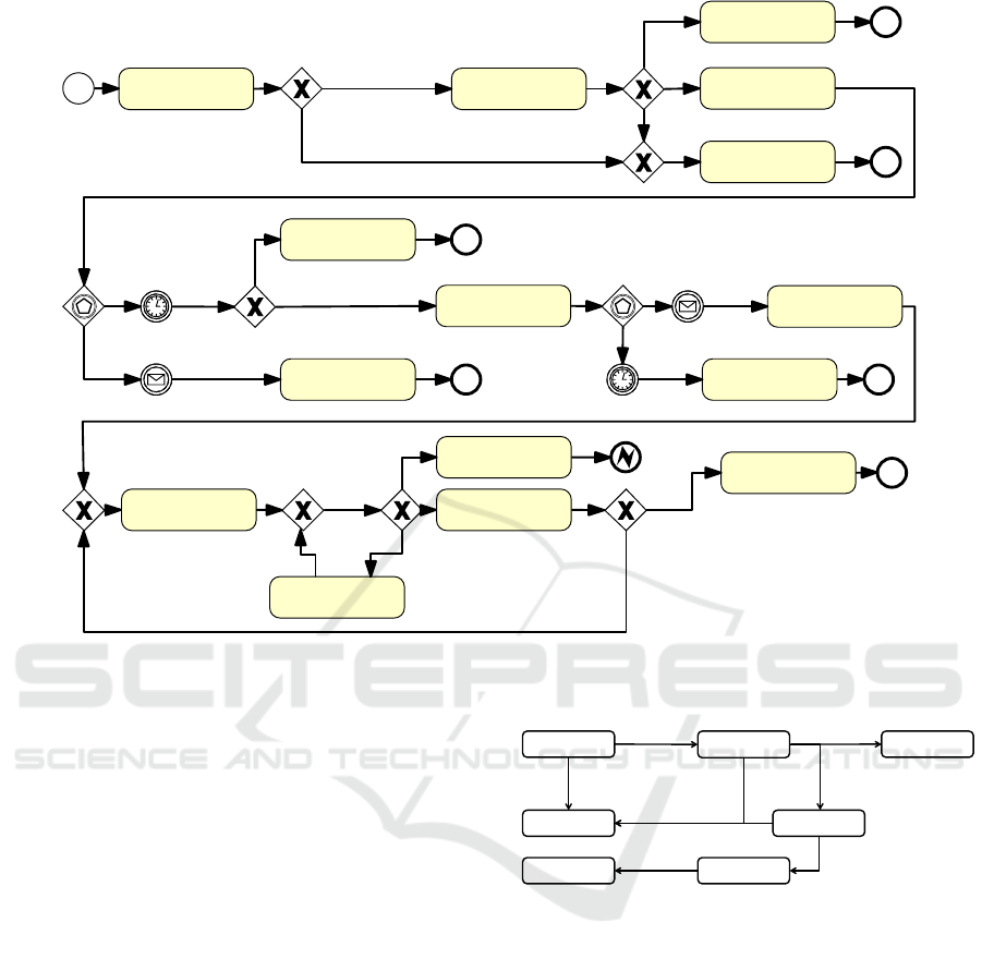
Figure 1 shows the process of booking and driving
a journey. During booking, a user enters the details of
the planned journey, including start and end station,
begin and end time, as well as destinations or kilome-
ters to drive. Then the system searches for alternatives
to fulfill this booking. Using a route calculation ser-
vice (Shekelyan et al., 2014), alternative routes and
vehicles are taken into account to find a possible al-
ternative to fulfill the request. If no alternatives are
found (e.g. if no free vehicles for the booking time are
left), booking is aborted. The user may select one of
the alternatives, which is then reserved. The user may
then abort or abandon the booking process. If the user
confirms the booking, it is added to the schedule with
the selected alternative. Note that at this point in time
no specific vehicle is promised to the user yet. Rather,
the reservation will be kept in the schedule, but may
be moved between equivalent vehicles if necessary.
The user may cancel the booking any time before it
starts.
At a defined time before the journey starts, all trips
are fixed to a suitable vehicle (at the correct location,
no other trips, sufficient charge), if one is available.
An interval of one hour was chosen as a trade-off
between optimization potential and user acceptance.
Up to this point the schedule optimizer may switch
vehicles if necessary. Note that existing bookings
are prioritized over new bookings, so no intentional
overbooking takes place. A vehicle will definitely
be available if no delays or malfunctions in previ-
ous bookings have occurred. If no vehicle is avail-
able, the booking is impossible and the user is noti-
fied. Otherwise, the user is sent a notification indi-
cating which vehicle to use including a virtual key to
unlock it. If the user starts the journey, he checks in
via an app. Then, he performs all trips in the journey
in order. During trips delays and malfunctions may
occur, which are communicated in real-time by the
vehicle (Ostermann et al., 2014) and may necessitate
changes in the schedule, as they may impact follow-
ing trips with the same vehicle. Finally, after the last
trip, the user checks out to finish the booking.
4 DYNAMIC OPTIMIZATION
In general, schedule optimization is a problem of se-
lecting which trips are to be performed by which ve-
hicles. This is a variant of the fixed interval schedul-
ing problem (Kovalyov et al., 2007) with additional,
usage scenario specific constraints. The schedule op-
timization aims to optimize a schedule in terms of a
SFFEV 2016 - Special Session on Simulation of flex fuel engines and alternative biofuel vehicles
254
Search booking
alternatives
1 hour before start
Cancellation
Suitable vehicle available?
Check in
End of booking period
Last trip of the booking
Found alternatives?
Mark booking no
show
Reserve booking
Timeout
Confirm booking
Abort booking
Cancel booking
Fix booking to
vehicle
Booking impossible
Start booking
Start trip
Vehicle malfunction
Trip delay
Finish trip
Finish booking
Yes
No
No
Yes
Yes
No
Figure 1: Main booking and driving process in Business Process Model and Notation (BPMN) 2.0.
goal function within existing constraints.
As a basis for optimization, we first describe the
relevant data types. Note that for the sake of brevity,
only attributes relevant for optimization are detailed
in this work.
A trip t ∈ T is a single step on a journey which
is performed with a single mode of transportation.
There are trips performed with fleet vehicles (T
f
) and
trips performed with external third party transporta-
tion (T
e
). For schedule optimization, external trips
t
e
∈ T
e
remain unchanged, as third party modes of
transportation cannot be influenced. The impact of
disruptions in third party transportation (e.g. late
trains) are currently ignored in schedule optimization
and subject for future work. A fleet trip is defined as
follows:
t ∈ T
f
:= (time
s
, time
e
, wp
s
, wp
e
, length)
where time
s
and time
e
are the start and end time,
wp
s
, wp
e
∈ WP the start and end waypoint and length
the length of the trip in kilometers. A waypoint
wp ∈ WP is a defined location like an address or ge-
olocation. A special kind of waypoint is a station
wp
station
∈ WP
station
⊂ WP, which belongs to the fleet
and offers parking as well as charging infrastructure.
A booking b ∈ B represents a journey a user plans
to undertake or has already made. It is defined as fol-
Reserved
Confirmed
Canceled
User confirms
User cancels
User aborts /
Timeout
Booking starts
in <= 1 hour &
no vehicle available
Fixed
Running
Finished
First trip starts
Last trip finishes /
Malfunction
Impossible
Booking starts
in <= 1 hour &
vehicle available
Figure 2: State diagram of bookings.
lows:
b ∈ B := (class, state, time
s
, time
e
,t
1
...t
n
)
where class is the desired vehicle class, state ∈
STATE
B
is the state of the booking, time
s
and time
e
are
the start and end time and t
1
...t
n
∈ T are a sequence
of trips in the booking (i.e. the journey). Note that a
journey has to start and end at a waypoint:
wp
s
t
1
, wp
e
t
n
∈ WP
station
Figure 2 shows a diagram of the booking states
STATE
B
and their relationships. A booking starts in
the state Reserved as soon as an alternative is se-
lected. This is to ensure the booking is still avail-
able when the user confirms, after which the book-
ing state is changed to Confirmed. One hour before
time
s
the booking is to be Fixed, i.e. for each trip
t
1
, ..., t
n
of the booking a vehicle is locked in. If not
Real-Time Schedule Optimization in Shared Electric Vehicle Fleets
255

all trips can be fixed, the booking state is changed to
Impossible. At any time before t
1
begins with check-
in, the user may abort or cancel the booking, which is
changed to the state Canceled. As t
1
begins, the book-
ing state changes to running. At this point it cannot be
canceled or changed by schedule optimization. After
t
n
has ended or a malfunction occurs, the booking is
eventually finished.
A vehicle v ∈ V is a fleet vehicle, which may ei-
ther be an EV or a conventional vehicle. In this work,
we focus on EVs, as conventional vehicles can be han-
dled as an EV with infinite range and without the need
of charging. We define a vehicle as follows:
v ∈ V := (class, em, oc, range,rcp)
where class is the vehicle class, em are the CO
2
emis-
sions per km in g, oc is the operating cost per kilo-
meter, range is the range in kilometers and rcp is
the recharging percentage per minute. We approxi-
mated charging curves linearly with a pessimistic es-
timate, so real-life charge will be at or above the es-
timated level. This approach was found sufficient
in (Sundstrom and Binding, 2010). Note that in our
prototype a uniform charging infrastructure at the sta-
tions is assumed, though in practice different charg-
ing modes can be faster or slower. This could be
amended by defining the available charging modes for
each w ∈ WP
station
.
A schedule E is a mapping of booking trips t ∈ T
f
to fleet vehicles v ∈ V as follows:
E := {(t,v)|t ∈ T
f
, v ∈ V ∪ {ε}}
Note that a trip may be mapped to no vehicle (ε).
These trips are unscheduled:
T
unscheduled
:= {t|∃(t, ε) ∈ E}
For each vehicle, a vehicle schedule E
v
is defined
as follows: E
v
:= {(t,x) ∈ E|x = v}
The set of all trips scheduled to a vehicle are de-
fined as follows: T
v
:= {t|∃(t, v) ∈ E}
A goal function z calculates the utility of a sched-
ule: z : E → R
During optimization, the utility of partial sched-
ules must be calculated. To achieve linear scalability
in regards to schedule size, a goal function needs to
fulfill the following independence criterion:
∀E : z(E) =
∑
(t,v)∈E
z({(t, v)})
This criterion stipulates that the utility of a sched-
ule is the sum of the utility of each trip. This allows
fast calculation of total utility when partial schedules
are merged by adding the utility of the partial sched-
ules.
Depending on the business goals of a car fleet op-
erator, different goal functions may be used, which
are detailed in (Koetter, 2015a). One example is the
minimization of CO
2
:
z(E) =
∑
(t,v)∈E
(−1 ∗ length
t
∗ em
v
)
Note that for this goal function the optimum is
reached when no trips are performed, as no CO
2
will
be produced. To avoid this unwanted result, the op-
timized schedule needs to fulfill a number of con-
straints:
The satisfiability constraint (C1) stipulates gen-
eral consistency and plausibility conditions.
∀v ∈ V : ∃t
1
, .., t
n
∈ T
v
: (∀t ∈ T
v
: t ∈ t
1
, ..., t
n
∧
length
t
≤ range
v
)∧ (∀i ∈ 1..n − 1 : time
e
t
i
+ buffer ≤
time
s
t
i
+1
∧ wp
e
t
i
= wp
s
t
i
+1
)
Each vehicle schedule has to be a sequence of
trips, which do not overlap in time and have at least
mathitbu f f er time between them. Each trip has to
start where the last ended and no trips’ length may
exceed the range of a vehicle.
Additionally, each trip must be mapped to exactly
one or no vehicle:
∀t ∈ T
f
: |(t, x)| ≤ 1
Similarly, the charge satisfiability constraint (C2)
stipulates sufficient charge must be available at all
times. Given a consistent trip sequence t
1
, .., t
n
for a
vehicle v as defined in C1, C2 is defined as follows:
∀t
i
∈ T
v
, i ∈ 2..n : length
t
i
≤ range
v
+
∑
j=1..i−1
(rcp
v
∗ (time
s
t
j
+1
− time
e
t
j
+ buffer)) −
length
t
j
)
Before each trip t
i
sufficient state of charge (SoC)
needs to be available in v, if previous trips are consid-
ered and standby times are used for charging.
The booking consistency constraint (C3) stipu-
lates that trips must match the selected booking de-
tails, including route and vehicle class.
Two constraints cannot always be fulfilled: The
fixing constraint (C4) stipulates that a trip has to be
performed by a fixed vehicle if it was already com-
municated to the user.
The completeness constraint (C5) stipulates that
all (or as many as possible) trips shall be mapped to
vehicles (T
unscheduled
=
/
0).
If these constraints cannot be fulfilled, C5 takes
precedence over C4.
To perform schedule optimization, a three-step al-
gorithm is used. An alternative search tries to fit a
new booking, a partial optimization optimizes only
the schedule of a single vehicle, while a full optimiza-
tion optimizes the whole schedule if necessary.
4.1 Partial Optimization
Partial optimization rearranges only the trips of a sin-
gle vehicle schedule and can be performed quickly,
thus enabling immediate user feedback (e.g. during
the booking process). Partial optimization is used if a
booking is performed or cancelled, if real-time infor-
mation about vehicle delays or malfunctions arrives
SFFEV 2016 - Special Session on Simulation of flex fuel engines and alternative biofuel vehicles
256

or if a vehicle is not returned on time. Partial opti-
mization for a vehicle v is performed as follows:
1. Order T
v
by time
s
to get a sequence t
1
, .., t
n
2. For i ∈ 1..n
(a) Try adding (t
i
, v) to E
v
considering vehicle state
taking into account current delays, malfunc-
tions and estimated charge at return
(b) If constraints C1-C3 are fulfilled, add (t
i
, v) to
E
v
new
(c) Else add (t
i
, ε) to T
unscheduled
3. Replace old vehicle schedule E
v
with E
v
new
Note that trips of running and fixed bookings are
added first due to chronological ordering. Also note
that partial optimization may violate constraint C5.
A vehicle state is updated whenever real-time data
arrives and has the following attributes: The avail-
ability of the vehicle indicates if a trip is currently
performed. The estimated remaining charge gives an
estimated SoC for the time the vehicle finishes its cur-
rent trip. It is used instead of range when evaluating
C2. The estimated return time gives an estimated time
of the vehicles arrival at wp
e
of its current trip. It is
used instead of time
e
for all constraints and further
calculations. If the vehicle is late or has less SoC than
anticipated, it is possible the following trips cannot be
scheduled to the vehicle without violating constraints.
4.2 Full Optimization
Full optimization is performed periodically in the
background by a scheduler. The optimization algo-
rithm as well as the goal function is encapsulated us-
ing interfaces. Though other algorithms are possible,
for the prototype we implemented a greedy algorithm:
1. Create an empty Schedule E
opt
:=
/
0
2. Sort all bookings b and vehicles v by vehicle class
3. For each class
(a) Sort all bookings b by state
b
(b) Add trips of completed and running bookings
to previously assigned vehicle, as they cannot
be reassigned anymore
(c) Fixed, confirmed and reserved bookings may
be optimized in this order
(d) Separate trips t of optimizable bookings in time
chunks TC (e.g. 1 day) by time
e
(e) For each time chunk TC
i. Calculate optimal subschedule E
sub
for all v
with class and t ∈ TC using a backtracking al-
gorithm
ii. Add optimized subschedule to optimized
schedule. E
opt
:= E
opt
∪ E
sub
4. Compare old and optimized schedule to select
E
new
(a) If E
opt
does not fulfill C1-C3: E
new
:= E
old
(b) Else if E
opt
does not fulfill C5 and E
old
does:
E
new
:= E
old
(c) Else if E
opt
does fulfill C5 and E
old
does not:
E
new
:= E
opt
(d) Else if both E
opt
and E
opt
fulfill C5:
i. If z(E
opt
) > z(E
old
): E
new
:= E
opt
ii. If z(E
old
) ≤ z(E
opt
): E
new
:= E
old
(e) Else if both E
opt
and E
opt
do not fulfill C5:
i. If |T
unscheduled
opt
| > |T
unscheduled
old
|: E
new
:=
E
opt
ii. If |T
unscheduled
opt
| ≤ |T
unscheduled
old
|: E
new
:=
E
old
5. Return E
new
This optimization algorithm uses a recursive step
to calculate optimal subschedules E
opt
, which is de-
tailed in the following:
1. Subschedule optimization is called with a se-
quence of trips t
1
, .., t
n
∈ TC, an existing schedule
E
opt
, a set of Vehicles V
class
and an initial utility u,
which is equal to z(E
opt
)
2. Determine initial vehicle state for all v ∈ V from
current state and trips in E
opt
3. Initialize choice list cl :=
/
0
4. ∀v ∈ V
class
(a) Test if t
1
can be added to v without violating
constraints
(b) If yes:
i. E
opt
:= E
opt
∪ {(t
1
, v)}
ii. Calculate utility and add it to total utility:
u
0
:= u + z({(t
1
, v)})
iii. Recursively call subschedule optimization
with t
2
, ..., t
n
, E
opt
, V
class
and u
0
iv. Add returned utility and mapping to choice list
: cl := cl ∪ (u
new
, (t
1
, v))
v. E
opt
:= E
opt
\ {(t
1
, v)}
5. Select best mapping m
opt
:= (t, v) where
(u, (t, v)) ∈ cl and u = max({u|∃(u, x) ∈ cl})
6. Add best mapping to optimized schedule: E
opt
:=
E
opt
∪ {m
opt
}
7. Calculate new utility: u
new
:= u + z({m
opt
})
8. Return u
new
and E
opt
Real-Time Schedule Optimization in Shared Electric Vehicle Fleets
257

Full optimization uses backtracking to recursively
calculate optimized timeline chunks. While the run-
time of backtracking is exponential, due to the con-
stant size of timeline chunks, an overall linear run-
time is achieved (for further details see (Koetter et al.,
2013)). An approximate optimum is created by com-
bining these local optima. Completed and running
trips cannot change vehicle anymore, fixed trips have
priority in the greedy algorithm. Only if they don’t fit
in the schedule of the fixed vehicle, are they moved.
After fixed trips have been distributed, confirmed trips
and reserved trips are distributed. This allows maxi-
mal optimization potential with minimal disruptions
to end users.
4.3 Alternative Search
During alternative search, alternatives for the re-
quested booking and all provided routes are searched
as follows:
1. Get a set of routes R := {(t
1
, .., t
n
)} for alternative
request from external route search
2. Intialize set of alternatives: A :=
/
0
3. For each r ∈ R
(a) Use subschedule calculation with all vehicles in
the requested vehicle class, the trips in r and a
copy of E to create E
new
(b) If ∀t ∈ r : (t, ε) 6∈ E
new
i. Add route as alternative: A := A ∪r
4. Return a
An alternative is found if the trips of a booking can
fit the current schedule while fulfilling all constraints.
As an immediate answer to the alternative search re-
quest is required to continue the booking process, the
search time needs to be minimized. Moving existing
trips to fit the alternative requires longer search times,
as no old bookings may be removed to fit the new al-
ternative. Thus, existing trips are not moved during
alternative search.
5 PROTOTYPE AND
EVALUATION
We implemented the algorithms for booking, alter-
native search, partial and full optimization in a Java
prototype, which we evaluated with synthetic tests as
well as in three long-term model trials with end users.
The schedule optimization prototype is part of the
larger Shared E-Fleet architecture (Ostermann et al.,
2014) and provides its services to a combined user
and administration frontend, while using third-party
route search (Shekelyan et al., 2014).
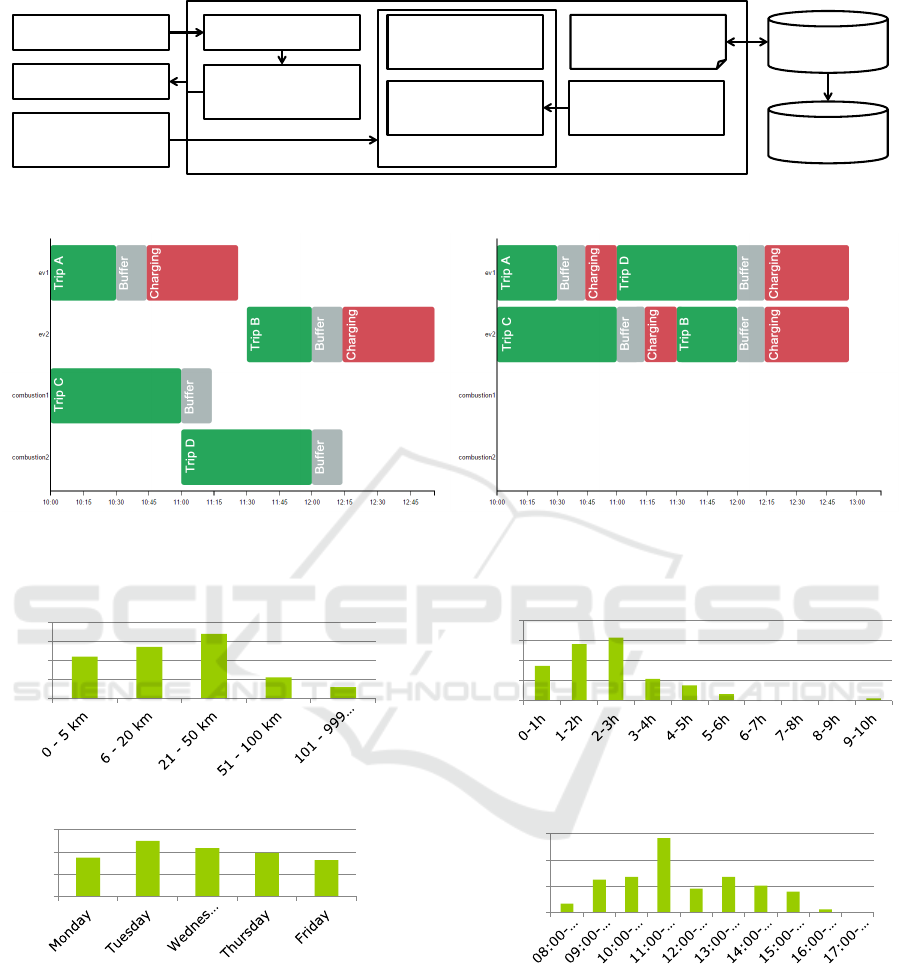
Figure 3 shows the architecture of the prototype.
A booking component provides booking functional-
ity to the frontend, while in turn using the alterna-
tive search algorithm to find alternatives for booking
requests. The optimizer contains algorithms for par-
tial and full optimization. If a real-time notification
about delays, malfunctions, returns, etc. is received,
the state of the respective EV is updated and a par-
tial optimization is performed. The scheduler periodi-
cally fixes trips, removes timed-out reserved bookings
and triggers full optimization. All components use the
schedule as a shared data-structure, which is read- or
write-locked when in use. The schedule is stored in
a database, from which it is reread if the prototype is
restarted. To improve run-time, completed and can-
celled trips are periodically moved to an archive, so
only current and future trips need to be handled dur-
ing optimization. Technical details of the prototype
can be found in a technical report (Koetter, 2015a).
We tested the prototype using randomly-generated
synthetic test-data and self-validation of consistency
and constraints. First trials showed a high utilization
of vehicles to be possible, provided journeys take half
a day or less.
Figure 4 shows an example schedule before and
after optimization. The car fleet consists of two
conventional vehicles, combustion1 and combustion2,
and two EVs, ev1 and ev2. Before optimization, four
trips are distributed equally among vehicles. Note
that conventional vehicles do not have charging times.
During optimization, the goal of CO
2
minimization is
considered. As EVs produce less CO
2
, they are pri-
oritized and two trips are scheduled to each. Note
that both vehicles cannot be fully charged after the
first trip, which leads to prolonged charging times af-
ter the second trip compared to the schedule previous
to optimization.
5.1 Model Trials
We further evaluated the prototype during three model
trials with a fleet of eight BMW i3 vehicles. Vehicles
were made available to technology parks for a year
to be used by real-life small and medium enterprises.
During model trials, we continuously improved the
algorithm under real conditions. While vehicles pro-
vided a range of over 100 kilometers, users tended to
book journeys with less than 50 kilometers and less
than 3 hour duration, as shown in Figure 5. Thus,
a potential for optimization was given. We found
64 percent of trips to be performed without any re-
optimization. Of the remaining 36 percent trips differ-
SFFEV 2016 - Special Session on Simulation of flex fuel engines and alternative biofuel vehicles
258
Frontend
Route search
Real-time
notifications
Booking
Alternative
search
Full
Optimization
Partial
Optimization
Schedule
Scheduler
Optimizer
Schedule
Archive
Figure 3: Overview of prototype architecture and control flow.
Figure 4: Example schedule before (left) and after optimization (right). Trips in green, buffer times in grey, charging times in
red.
© Shared E-Fleet Konsortium 1
0%
10%
20%
30%
40%
Distribution by journey duration
Distribution by journey distance
0%
10%
20%
30%
40%
Distribution by weekday Distribution by time of day
0%
10%
20%
30%
0%
10%
20%
30%
Figure 5: Statistical evaluation of model trial in Stuttgart.
ent causes necessitated a re-optimization. We found
users to be optimistic regarding their planned return
times, as cars would often be returned late, necessi-
tating re-optimization. During partial optimization,
the following trip would be removed from the vehi-
cle schedule and then added to a different vehicle’s
schedule during full optimization. Often, the follow-
ing trip was already fixed, making an additional no-
tification to the user necessary, as the vehicle change
needed to be communicated. We found the earlier and
the more precise delays can be detected and commu-
nicated by the vehicle, the better the planning and in
turn the end-user experience. Another scenario for
re-optimization was the cancellation of bookings by
users, which occurred for about 13 percent of book-
ings. In addition, hardware problems at the beginning
of the model trials necessitated the temporary removal
of single cars from the fleet. Schedule optimization
proved to allow business continuity and quality of ser-
vice in spite of these disruptions.
Real-Time Schedule Optimization in Shared Electric Vehicle Fleets
259
Setup
Simulation
Request count
reached?
Create random
booking
request
Attempt
booking
Booking
successful?
Full
optimization
Full optimization
activated?
Calculate
schedule
statistics
no
yes
yes
no
no
yes
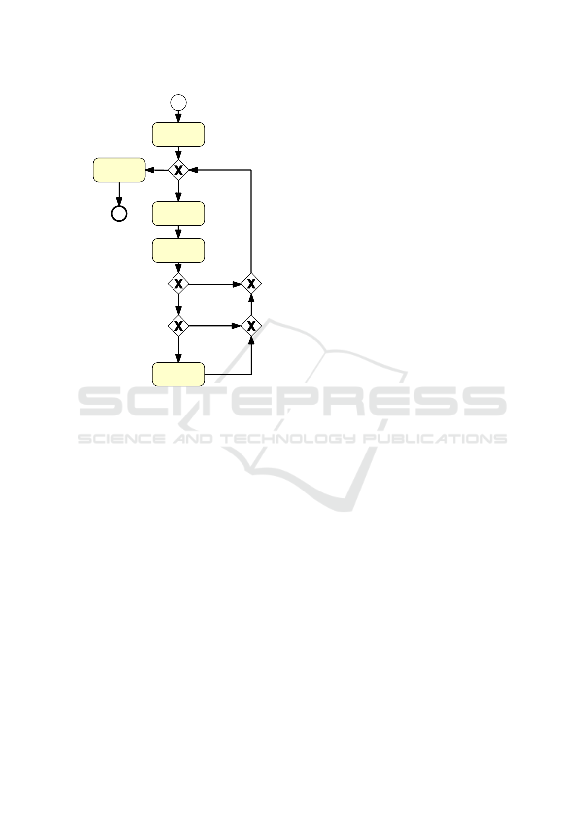
Figure 6: Schedule optimization benchmark process in
BPMN 2.0.
further model trials are currently still running, this
time using heterogeneous fleets, to further investigate
the impact of schedule optimization on CO
2
and cost.
5.2 Synthetic Evaluation
While model trials provide insights into schedule op-
timization in practice, they are not sufficient for quan-
titative evaluation. As all parts of the system are eval-
uated simultaneously, many influences and variables
cannot be controlled. For example, hardware prob-
lems unrelated to schedule optimization provide in-
sights into rescheduling in face of disruptions, but
distort many metrics like goal fulfillment. Thus, we
performed an additional evaluation with synthetic test
data.
For this evaluation, a benchmark tool was built to
interface with the schedule optimization. The bench-
mark process is shown in Figure 6. During setup an
empty schedule is created according to the benchmark
settings. These settings include:
• Business hours: Which hours of the day are busi-
ness hours? (e.g. 7:00-17:00)
• Number of requests: How many booking requests
are to be attempted?
• Seed: A seed for pseudorandom booking genera-
tion.
• Time interval: The time interval of the trial within
which requests are to be generated. (e.g. October
1st 2016 0:00 to November 1st 2016 0:00)
• Use full optimization: Whether or not full opti-
mization is to be used.
• Goal function: The goal function to be used.
(minimizing emissions or cost)
• Vehicle fleet: The fleet to be used.
• Customer profile: Determines how booking re-
quests are generated.
During the benchmarks booking requests are cre-
ated according to a customer profile. The profile used
creates booking requests within the business hours,
using the following length and duration:
lengthKM = Math.max(10.0,
((25.0 * rand.nextGaussian()) + 25))
durationMinutes = rand.nextInt(211) + 30
To investigate the effect of schedule optimization
regarding goal functions, heterogeneous fleets, con-
sisting of both conventional vehicles and EVs are
used. The vehicles are shown in Table 1. As conven-
tional vehicles, data of three representative vehicles
is used (Deffner and Goetz, 2012). For EVs, data of
three common vehicles is used (Bloch, 2014). Prices
and emissions are calculated using average fuel prices
and wind energy (Deffner and Goetz, 2012). CO
2
emissions for EVs are calculated from emissions oc-
curing during energy production. Note that charging
rates are for regular charging, which is available at
any station. The possibility of DC charging was not
considered as it was not available during the model
trials. However, faster charging times can increase
fleet utilization. In the evaluation, three fleets are used
as listed in Table 2. Regardless which fleet is evalu-
ated, the benchmark uses one central station at which
all trips begin and end.
After setup, the benchmark tool creates synthetic
bookings from the customer profile using a fixed ran-
dom seed, making the benchmark process repeatable.
Each booking is attempted to be booked by searching
for alternatives and booking the best alternative. Note
that exactly one route will be generated, as only a flat
distance is specified. If no alternatives are found, the
booking cannot be completed, indicating a lack of va-
cancies in the schedule. If full optimization is to be
used, it is performed after each successful booking. If
the specified number of requests has been attempted,
the benchmark concludes with calculating the statis-
tics of the resulting schedule.
SFFEV 2016 - Special Session on Simulation of flex fuel engines and alternative biofuel vehicles
260

Table 1: Benchmark vehicle data.
Model Type
Cost in e / km
g CO
2
/ km
Battery Capacity in kWh
Consumption in kWh / 100 km
Recharged kWh / hour
CombustionLarge Conventional 0.152 272.000 — — —
CombustionMedium Conventional 0.113 200.000 — — —
CombustionSmall Conventional 0.089 159.000 — — —
Tesla Model S Electric 0.092 8.064 85.00 33.60 3.03
BMW i3 Electric 0.057 4.944 22.00 20.60 2.75
Renault Twizy Electric 0.032 2.808 7.00 11.70 2.33
Table 3: Benchmark for large fleet and medium number of requests.
Optimization strategy Random Random Emission Emission Cost Cost
Use full optimization false true false true false true
Fulfilled bookings 491 493 489 488 489 488
Unfulfilled bookings 9 7 11 12 11 12
Total kilometers 12329,00 12395,00 12301,00 12271,00 12301,00 12318,00
Total CO
2
in kg 1462,79 1557,56 975,18 719,17 1024,38 844,63
Total cost in e 1066,60 1099,79 919,38 844,00 918,13 842,54
Total usage hours 309,00 309,00 309,00 309,00 309,00 309,00
Fleet utilization 34,572 34,891 34,487 34,509 34,487 34,524
CO
2
per km in g 118,65 125,66 79,28 58,61 83,28 68,57
Cost per km in e 0,0865 0,0887 0,0747 0,0688 0,0746 0,0684
Full opt. gain Util. gain % 0,92 CO
2
saved % 35,27 Cost saved % 9,12
Partial opt. gain — — 49,66 114,41 15,91 29,72
Table 2: Benchmark vehicle fleets.
Model
Small Fleet
Medium Fleet
Large Fleet
CombustionLarge 0 1 1
CombustionMedium 2 1 2
CombustionSmall 0 1 2
Tesla Model S 0 1 1
BMW i3 2 1 2
Renault Twizy 0 1 2
Multiple benchmarks have been performed with
all possible combinations of the following settings:
• Number of requests:
– Low: 1 request per vehicle per day
– Medium: 2 requests per vehicle per day
– High: 4 requests per vehicle per day
– Very high: 8 requests per vehicle per day
• Use full optimization: Yes or No
• Goal function: Random, Minimize Cost or Mini-
mize Emissions
• Vehicle fleet: Small, Medium or Large
Table 3 shows the full results for a large fleet and
medium utilization. Detailed results can be found in
a technical report (Koetter, 2015b). Full test input
and result data can be found online
3
. An overview
of benchmark results is given in Figure 7. Optimiza-
tion potentials for emissions and costs rise with lower
utilization, as more bookings can be moved to opti-
mal vehicles, e.g. with low utilization most trips can
be moved to EVs to minimize emissions. With higher
3
www.shared-e-fleet.de/images/sefevaluation raw data.zip
Real-Time Schedule Optimization in Shared Electric Vehicle Fleets
261
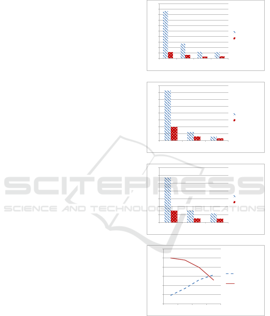
utilization, lower potentials can be realized, as even
suboptimal vehicles need to be used. Optimization
potentials with low utilization are very high but would
not be practical, as in such cases vehicles should be
removed from the fleet to save additional fixed costs.
High utilization allows emission savings of 25-30 per-
cent, and cost savings of 7-11 percent. Very high uti-
lization allows emission savings of 11-23 percent and
cost savings of 6-10 percent.
When only using partial optimization, savings are
lower throughout the benchmarks. With high and
very high utilization, using partial optimization actu-
ally produces worse results than no optimization at
all. This is because the greedy approach of partial op-
timization achieves early gains and fills optimal vehi-
cles, leaving only small gaps for later bookings. With-
out full optimization, these cannot be filled and a dis-
proportionate amount of trips are booked on subop-
timal vehicles, thus producing suboptimal schedules.
This indicates partial optimization alone is not suffi-
cient for schedule optimization, validating the three-
step approach described in this work.
the utilization of a fleet indicates the percentage
of time vehicles are in use during business hours. The
diagram in the bottom right of Figure 7 shows the re-
lation between utilization and successful booking at-
tempts. The more a schedule is filled, the less va-
cancies remain for future bookings. Thus, with ris-
ing utilization, booking is less and less successful. In
practice, a success rate of only fifty percent means ev-
ery second user is denied a booking request, leading
to low user acceptance. Considering a success rate
of 80 percent as acceptable, a utilization of about 55
percent is achievable.
Fleet utilization is almost constant between dif-
ferent optimization strategies, differing by less than
one percent. This however is not true for a very
high number of requests, where utilization is 2-10
percent lower if full utilization is used. This is be-
cause full optimization moves trips with more kilo-
meter to electric vehicles if possible, necessitating
recharging times during the day, especially if multiple
bookings on the same day are scheduled to the same
vehicle. These charging times lower utilization, as
they block the vehicle for additional trips. In compar-
ison, scheduling bookings randomly distributes long
trips more evenly, achieving higher utilization at the
cost of the optimization goal. Further research in this
phenomenon could improve the algorithm depending
on the priorities of a car fleet operator.
(1) Optimization potential in small fleet
(4) Utilization and service level
0%
20%
40%
60%
80%
100%
120%
140%
160%
180%
200%
low
utilization
medium
utilization
high
utilization
very high
utilization
emission savings %
cost savings %
0%
20%
40%
60%
80%
100%
120%
140%
160%
medium
utilization
high utilization very high
utilization
emission savings %
cost savings %
(2) Optimization potential in medium fleet
0%
20%
40%
60%
80%
100%
120%
140%
medium
utilization
high utilization very high
utilization
emission savings %
cost savings %
0,00%
20,00%
40,00%
60,00%
80,00%
100,00%
120,00%
low
utilization
medium
utilization
high
utilization
very high
utilization
Utilization
% booking requests
fulfilled
(3) Optimization potential in large fleet
Figure 7: Overview of benchmark results.
6 CONCLUSION AND OUTLOOK
In this work, we describe processes and algorithms for
dynamic real-time schedule optimization, allowing a
SFFEV 2016 - Special Session on Simulation of flex fuel engines and alternative biofuel vehicles
262

high utilization of electrical car fleets, a compensa-
tion of disruptions and malfunctions and an economic
and ecological optimization of operations. We imple-
mented these techniques in a prototype and evaluated
them in long-term model trials with real users as part
of a fleet management system as well as in a bench-
mark, showing considerable savings can be achieved.
In future work, we would like to further enhance
optimization algorithms and evaluate them with het-
erogeneous vehicle fleets in additional model trials.
ACKNOWLEDGEMENTS
This research has been supported by the IKT II pro-
gram in the Shared E-Fleet project. They are funded
by the German Federal Ministry of Economics and
Technology under the grant number 01ME12105.
The responsibility for this publication lies with the au-
thors.
REFERENCES
Bielli, M., Bielli, A., and Rossi, R. (2011). Trends in mod-
els and algorithms for fleet management. Procedia-
Social and Behavioral Sciences, 20:4–18.
Bloch, A. (2014). E-autos im h”artetest (in german). Auto,
Motor und Sport, 16. http://www.auto-motor-und-
sport.de/vergleichstest/elektroautos-6-modelle-im-
haertetest-8498096.html.
Deffner, Jutta, B.-H. B. H. T. and Goetz, K. (2012).
Elektrofahrzeuge in betrieblichen Fahrzeugflot-
ten - Akzeptanz, Attraktivitt und Nutzungsver-
halten (in German). ISOE-Studientexte, 17.
http://www.isoe.de/uploads/media/st-17-isoe-
2012.pdf.
del Razo, V., Goebel, C., and Jacobsen, H.-A. (2014).
Benchmarking a car-originated-signal approach for
real-time electric vehicle charging control. In Inno-
vative Smart Grid Technologies Conference (ISGT),
2014 IEEE PES, pages 1–5. IEEE.
Koetter, F. (2015a). Dynamische Einsatzopti-
mierung von gemeinsam genutzten Elektro-
fahrzeugflotten (in German). http://www.shared-e-
fleet.de/images/Dynamische Einsatzoptimierung von
gemeinsam genutzten Elektrofahrzeugflotten.pdf.
Koetter, F. (2015b). Evaluation of Dynamic
Schedule Optimization. http://www.shared-e-
fleet.de/images/evaluation schedule optimization.pdf.
Koetter, F., Klausmann, F., and Renner, T. (2013). Poten-
zialermittlung f
¨
ur integration von elektrofahrzeugen
in fuhrparkflotten. Informatik-Spektrum, 36(1):35–45.
Kovalyov, M. Y., Ng, C., and Cheng, T. E. (2007). Fixed
interval scheduling: Models, applications, computa-
tional complexity and algorithms. European Journal
of Operational Research, 178(2):331–342.
Ostermann, J., Renner, T., Koetter, F., and Hudert, S.
(2014). Leveraging electric cross-company car fleets
through cloud service chains: The shared e-fleet ar-
chitecture. In Global Conference (SRII), 2014 Annual
SRII, pages 290–297. IEEE.
Pillac, V., Gendreau, M., Gu
´
eret, C., and Medaglia, A. L.
(2013). A review of dynamic vehicle routing prob-
lems. European Journal of Operational Research,
225(1):1–11.
Pl
¨
otz, P., Gnann, T., K
¨
uhn, A., and Wietschel, M. (2013).
Markthochlaufszenarien f
¨
ur elektrofahrzeuge. Karl-
sruhe: Fraunhofer-Institut f
¨
ur System-und Innova-
tionsforschung ISI.
Sassi, O. and Oulamara, A. (2014). Joint scheduling and op-
timal charging of electric vehicles problem. In Com-
putational Science and Its Applications–ICCSA 2014,
pages 76–91. Springer.
Shekelyan, M., Joss
´
e, G., Schubert, M., and Kriegel, H.-P.
(2014). Linear path skyline computation in bicriteria
networks. In Database Systems for Advanced Appli-
cations, pages 173–187. Springer.
Sundstrom, O. and Binding, C. (2010). Optimization Meth-
ods to Plan the Charging of Electric Vehicle Fleets.
Real-Time Schedule Optimization in Shared Electric Vehicle Fleets
263
