Comparing Machine Learning Techniques in a
Hyperemia Grading Framework
L. S. Brea
1
, N. Barreira
1
, A. Mosquera
2
, H. Pena-Verdeal
3
and E. Yebra-Pimentel
3
1
Department of Computer Science, Univ. A Coruna, A Coru˜na, Spain
2
Department of Electronics and Computer Science, Univ. Santiago de Compostela, Santiago de Compostela, Spain
3
Department of Applied Physics, Univ. Santiago de Compostela, Santiago de Compostela, Spain
Keywords:
Image Processing, Medical Imaging, Pattern Recognition.
Abstract:
Hyperemia is the occurrence of redness in a certain tissue. When it takes place on the bulbar conjunctiva,
it can be an early symptom of different pathologies, hence, the importance of its quick evaluation. Experts
grade hyperemia as a value in a continuous scale, according to the severity level. As it is a subjective and
time consuming task, its automatisation is a priority for the optometrists. To this end, several image features
are computed from a video frame that shows the patient’s eye. Then, these features are transformed to the
grading scale by means of machine learning techniques. In previous works, we have analysed the performance
of several regression algorithms. However, since the experts only use a finite number of values in each grading
scale, in this paper we analyse how classifiers perform the task in comparison to regression methods. The
results show that the classification techniques usually achieve a lower training error value, but the regression
approaches classify correctly a larger number of samples.
1 INTRODUCTION
Hyperemia is the occurrence of an abnormal hue of
red in a tissue. One of the areas that can be affected
is the bulbar conjunctiva, where it can be an early
symptom of pathologies such as conjunctivitis, aller-
gies, contact lens complications, or dry eye syndrome
(Rolando and Zierhut, 2001). Specialists measure hy-
peremia as a degree in a continuous scale. Scales
are collections of pictures or photographies that rep-
resent different levels of severity. The clinician com-
pares the patient’s eye with the images, and assigns a
level. In this paper, we work with two of the available
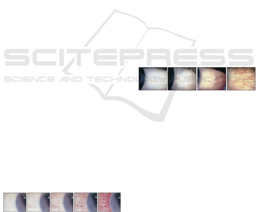
scales: Efron (5 levels of severity, shown in Fig. 1)
and CCLRU (4 levels, depicted in Fig. 2). Specialists
grade using not only the 4-5 prototype levels, but also
decimal values indicating how much a patient’s eye
distances from the model.
Figure 1: Efron severity levels. Photographic scale.
In order to perform the evaluation, experts take
into account several parameters. Some examples
Figure 2: CCLRU severity levels. Drawing scale.
are the general hue of the conjunctiva, the number
of blood vessels, or their width. The task is time-
consuming and presents high intra and inter expert
subjectivity. This arises the need of its automatisation.
There are few approaches that tackle the problem of
automatic hyperemia computation. Different frame-
works have been developed, but there are some steps,
such as the determination of the region of interest,
that are not automatic (Yoneda et al., 2012; Rodriguez
et al., 2013). There are several works that propose
features that need to be calculated in order to perform
the grading (Papas, 2000; Wolffsohn and Purslow,
2003). There are also different works that depict the
construction and validation of grading scales (Efron
et al., 2001; Fieguth and Simpson, 2002), analysing
how specialists tend to choose the values they assign.
One of the most important steps is the transfor-
mation from the image features to the grading scale
values. This transformation can be performed using
regression methods, as both the feature scale and the
Brea, L., Barreira, N., Mosquera, A., Pena-Verdeal, H. and Yebra-Pimentel, E.
Comparing Machine Learning Techniques in a Hyperemia Grading Framework.
DOI: 10.5220/0005756004230429
In Proceedings of the 8th International Conference on Agents and Artificial Intelligence (ICAART 2016) - Volume 2, pages 423-429
ISBN: 978-989-758-172-4
Copyright
c
2016 by SCITEPRESS – Science and Technology Publications, Lda. All rights reserved
423
expert grading are continuous. However, in practice
specialists do not use all the values in a continuous
scale, but have a tendency to assign certain grades
more frequently, such as integer and half-integer val-
ues (Schulze et al., 2007). Those values are taken
as references even when they assign other amounts.
This give us the possibility to apply classification al-
gorithms by performing an initial division of the val-
ues in classes. In this work, we analyse how classifier
methods are able to perform the transformation of the
image features into grading scale values. We compare
the results achieved by these methods to different re-
gression techniques.
The paper is structured as follows: Section 2 ex-
plains the approaches we have selected as well as the
experiments, Section 3 shows the results, and Sec-
tion 4 discusses the conclusions and future lines of
research.
2 METHODOLOGY
Specialists grade hyperemia by analysing a video of
the patient’s eye. For the automatisation of the pro-
cess, we receive this video as input and perform four
steps to obtain the value in the grading scale as the
output. First, the input video is analysed in order to
select the frame that is the most suitable for grading
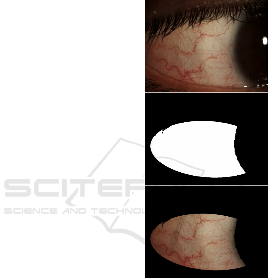
(S´anchez et al., 2015a). Then, a region of interest
comprising only the bulbar conjunctiva is delimited
by means of an elliptical mask and thresholding oper-
ations. It is depicted in Fig. 3 how the mask removes
the iris and pupil area, the eyelids, and the eyelashes.
Next, several image features are computed and, last,
these features are transformed into the grading value
(S´anchez et al., 2015b). This work is focused in the
final step of the process. This section presents the
image features we worked with as well as the classi-
fication and regression approaches used.
2.1 Feature Computation
Specialists take different parameters into account
when performing hyperemia grading. This way, ex-
pert knowledge is the first issue we have to face, as it
is difficult to explain and understand which features
are relevant. For example, the amount of red value
in the image implies a higher hyperemia level, but it
does not have the same relevance if that redness cor-
responds to vessel or background areas. We also have
to take into account the general tonality of the image,
as the illumination is not constant for all the image
set. This lead us to implement measures that com-
pare the red value to other colours. We have to simu-
Figure 3: Region of Interest of the conjunctiva.
late the expert perception so that we also test several
colour spaces, such as RGB, HSV, and L*a*b*, in or-
der to determine which one offers the best representa-
tion. Moreover,experts look at the vessel quantity and
width too, as hyperemia is produced by blood vessel
engorgement.
After consulting past works on the subject (Papas,
2000; Wolffsohn and Purslow, 2003) and talking to
optometrists, we computed 25 image features:
• Vessel count f
1
. The image is scanned horizon-
tally in ten rows equally separated and the number
of vessels that are cut is counted.
ICAART 2016 - 8th International Conference on Agents and Artificial Intelligence
424

• Vessel occupied area f
2
. The number of vessel
pixels is divided by the ROI size.
• Relative vessel redness f
3
and relative image red-
ness f
4
. (RGB) Sum of red channel values divided
by all the channels’ values for all the vessel pixels
or the whole image pixels, respectively.
• Difference red-green in vessels f
5
and in the im-
age f
6
(RGB). Sum of differences between red
and green channels divided by all the channels’
values for all the vessel pixels or the whole image
pixels, respectively.
• Difference red-blue in vessels f
7
and in the image
f
8
(RGB). Sum of differences between red and
blue channels divided by all the channels’ values
for all the vessel pixels or the whole image pixels,
respectively.
• Red hue value f
9
(HSV). Sum of the red compo-
nent of the hue channel for all the pixels divided
by the ROI size.
• Percentage of vessels f
10
. The number of vessel
pixels is divided by the total pixels and multiplied
by 100 as it was originally proposed in (Papas,
2000).
• Percentage of red in vessels (RGB f
11
, HSV f
12
).
Sum of red value for all the vessel pixels divided
by the number of vessel pixels.
• Redness in neighbourhood (HSV), f
13
. Besides
taking into accountthe current pixel, the hue value
is also analysed in the neighbouring pixels. The
whole image is analysed.
• a-channel in vessels f
14
and in the image f
15
(L*a*b*). Sum of the values of the a-channel in
each pixel corresponding with a vessel divided by
the ROI size, or sum through all the pixels of the
image.
• Yellow in background (RGB, HSV, L*a*b*) f
16
-
f
18
. Sum of yellow value for those pixels cor-
responding to conjunctiva (areas without vessels)
divided by the ROI size.
• Red in background (RGB, HSV, L*a*b*), f
19
-f
21
.
Sum of white value for those pixels corresponding
to conjunctiva divided by the ROI size.
• White in background (RGB, HSV, L*a*b*), f
22
-
f
24
. Sum of red value for those pixels correspond-
ing to conjunctiva divided by the ROI size.
• Vessel width, f
25
. Vessel widths are measured in
ten circumferences centered at the corner of the
eye and with radius ranging from h/2∗ n to h/2,
where h is the height of the image and n the num-
ber of circumferences, by means of an active con-
tour algorithm (V´azquez et al., 2013). The mean
vessel width is selected as the representative fea-
ture.
In features based on vessels, a Canny filter is applied
to locate the vessel boundaries (Canny, 1986). The
filter performance was previously evaluated by manu-
ally segmenting 106 vessels from our image set. 94%
of these vessels were correctly extracted by the auto-
matic method. In order to obtain the values for the
red hue in HSV, we measure the H-channel and check
the value |H − 128|, as H-channel range is 0 to 255
and the purest red is in 0 and 255. For a-channel in
L*a*b*, positive values mean that there is red hue,
while the negative ones correspond to green colour.
RGB values are directly obtained by accessing the ap-
propriate channel.
2.2 Hyperemia Grading
One of the most important and overlooked steps in
hyperemia grading is the transformation from the im-
age features to the grading scale. This procedure in-
volves finding the relationship between feature values
and the given scale. It was originally approached with
regression methods in (S´anchez et al., 2015b). Even
though both scales are in theory continuous, several
researches have study how in reality experts only ap-
ply a certain set of values in their gradings. Hence, in
this work we are applying classifier models and com-
paring its performance with regression methods.
Classifier models present certain benefits if com-
pared with regression techniques. For example, some
regression methods require to assume the data follows
a certain distribution or structure, such as linear re-
gression. Other more complex methods, like artificial
neural networks, model well convoluted relationships
but at the cost of being opaque. This is an issue spe-
cially when we are interested in understanding the un-
derlying relationship and not only in training a system
that achieves good predictions.
In order to apply classification techniques to con-
tinuous data, we need to group the values in classes.
The first decision we have to face is how to imple-
ment this division. We performed experiments with
three assumptions:
• Using integer and half-integer values. This ap-
proach is supported by those works that conclude
that experts usually grade taking this characteris-
tic values as a reference (Schulze et al., 2007).
• Using one decimal. This is the maximum preci-
sion of human experts when grading.
• Using integer, half and quarter values. We decided
to include this approach in order to check how the
values evolve with the gap between classes.
Comparing Machine Learning Techniques in a Hyperemia Grading Framework
425
For each of these assumptions, we applied a set of
classifiers, chosen in order to cover the different types
of machine learning algorithms:
• Bayes Network (BN) (Friedman et al., 1997;
Jensen, 1996).
• Naive Bayes (NB) (John and Langley, 1995).
• Support Vector Machine (SVM) (Chang and Lin,
2011).
• Sequential Minimal Optimisation (SMO) (Platt
et al., 1999; Keerthi et al., 2001; Hastie et al.,
1998).
• Instance Based (IB1 and IB3) (Aha et al., 1991).
• Decision Table (DT) (Kohavi, 1995).
• One Rule (OR) (Holte, 1993).
• Decision Tree (J48) (Quinlan, 2014).
• Random Forest (RF) (Breiman, 2001).
Regarding the regression methods we also se-
lected the following approaches:
• Instance Based (IBR) (Aha et al., 1991).
• Linear Regression (LR).
• Support Vector Regresion (SVR) (Smola and
Sch¨olkopf, 2004).
• M5P (Wang and Witten, 1996; Quinlan et al.,
1992).
• Multi Layer Perceptron (MLP) (Baum, 1988).
• Radial Basis Function Network (RBFN) (Buh-
mann, 2000).
3 RESULTS
Our data set consisted of 105 videos of the bulbar
conjunctiva. These videos have been filmed by the
Optometry Group (University of Santiago de Com-
postela) following a standardised acquisition proto-
col. The videos belong to different patients. Even
though each person could present a different distribu-
tion of vessels in the conjunctiva, a extremely high
number is considered unusual and labelled with high
values in the scale.
For each video, the best frame is selected, result-
ing in an image of 1024× 768 px that shows a side
view of the eye, from the pupil to the corner of the
eye or the lacrimal. The images had been graded by
two optometrists twice. The mean value for the two
gradings was computed for each specialist and then,
the mean value from both specialists is used as target.
Due to the subjectivity of the problem, it is difficult to
find how the expert’s gradings and the image features
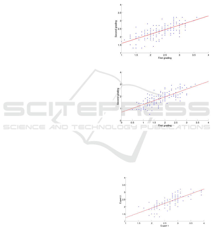
are related. Figures 4 and 5 depict the issue of the in-
tra expert subjectivity. Both gradings were performed
months apart, and we can observe how the given val-
ues vary. Moreover, this variation is not consistent, as
the expert assigned higher values on the second grad-
ing for the lower levels of severity but lower ones for
the most severe conjunctivas.
Figure 4: Intra expert differences in CCLRU scale.
Figure 5: Intra expert differences in Efron scale.
Figures 6 and 7 show the inter expert differences
in both scales. We can notice how the experts per-
form different when grading near the various levels
of severity. In fact, if we compare the gradings of
the two experts, we obtain a RMSE of 0.4705 for the
Efron scale and 0.4743 for the CCLRU scale.
Figure 6: Inter expert differences in CCLRU scale.
We divided the continuous output in classes sep-
arated a certain step (0.5, 0.25, and 0.1). The meth-
ods were trained using 10-fold cross validation. We
computed the success rate during the training. For the
ICAART 2016 - 8th International Conference on Agents and Artificial Intelligence
426
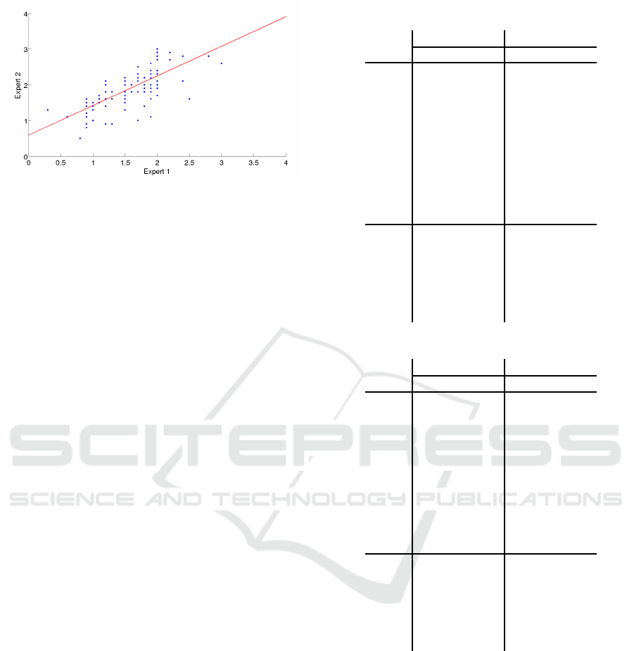
Figure 7: Inter expert differences in Efron scale.
regression methods, as they provide a continuous re-
sult, an instance was accounted as correctly classified
if the closest defined class to this output value was
the expected one. We used the data mining software
Weka (Hall et al., 2009). In order to select the pa-
rameters for each classifier, empirical tests were con-
ducted. The systems configurations were the follow-
ing:
• BN: search algorithm is K2 (Cooper and Her-
skovits, 1991). Alpha value for the estimator is
0.5.
• SVM: type = C-SVC, kernel = radial basis func-
tion.
• SMO: Pearson universal kernel (ω = 1.0, σ =
1.0).
• IB1: neighbours = 1.
• IB3: neighbours = 3.
• DT: the evaluation measure is the RMSE.
• J48: confidence factor for pruning = 0.25, mini-
mum instances per leaf = 2.
• RF: number of trees = 100.
• IBR: neighbours = 3.
• SVR: type = ε-SVR
• M5P: minimum instances per leaf = 4.
• MLP: hidden layers = [40 16], learning rate = 0.3,
training epochs = 500.
Tables 1, 2 and 3 depict the results obtained for
both scales and all the methods. The root mean
squared error (RMSE) was obtained during the train-
ing stage for the whole image set.
We can observe how the error value is higher as
the step becomes wider, but the number of correctly
classified images is also larger. This was expected,
as a misclassification generates a worse error when
the gap between values is broader. SMO classifier
achieves consistently good results. Some of the meth-
ods obtain a perfect classification on the test set in
some of the test cases, such as RF with step=0.25.
Table 1: Classification results (step=0.5).
Efron CCLRU
SR RMSE SR RMSE
BN 46.7 0.3073 53.3 0.3254
NB
38.1 0.3551 43.8 0.3755
SVM 41.9 0.3593 44.8 0.3973
SMO
48.6 0.286 56.2 0.3086
IB1 40.0 0.3651 51.4 0.3725
IB3
41.0 0.2959 44.8 0.3207
DT 46.7 0.2714 54.3 0.294
OR 35.2 0.3794 45.7 0.3938
J48
39.0 0.354 53.3 0.3401
RF 41.0 0.2751 58.1 0.2831
IBR 46.7 0.4213 56.2 0.353
LR
54.3 0.404 55.2 0.3478
M5P 47.6 0.3801 58.1 0.3224
MLP
36.2 0.4882 50.5 0.4223
RBF 40.0 0.4683 49.5 0.3809
SVR
41.9 0.4945 44.8 0.3997
Table 2: Classification results (step=0.25).
Efron CCLRU
SR RMSE SR RMSE
BN 20.0 0.2365 32.4 0.2701
NB 21.9 0.2816 31.4 0.2994
SVM
21.0 0.305 25.7 0.3381
SMO 21.0 0.2249 36.2 0.252
IB1 27.6 0.2918 31.4 0.3248
IB3
15.2 0.2441 24.8 0.2688
DT 21.0 0.2234 33.3 0.2463
OR
24.8 0.2975 25.7 0.3381
J48 28.6 0.2776 31.4 0.3052
RF
18.1 0.2264 35.2 0.246
IBR 25.7 0.3846 39.1 0.3006
LR 34.3 0.3753 28.7 0.2991
M5P
28.6 0.3772 34.3 0.2956
MLP 31.4 0.4465 35.2 0.3472
RBF
20.0 0.4433 25.7 0.3619
SVR 21.0 0.4722 25.7 0.3809
However, our main goal is to achieve a lower RMSE,
as the number of correctly and incorrectly classified
images can be misleading. For example, an overfitted
model will present good results in these parameters
but with a higher RMSE.
Regarding the differences between both types of
methods, we can perceive how the regression meth-
ods achieve, with the exception of SMO classifier,
better results, as they classify correctly a larger num-
ber of images. However, training error is higher also
for regression methods. This happens because almost
all regression predictions have at least a slight error,
since the model does not predict the exact output.
We also have to take into account that a high
Comparing Machine Learning Techniques in a Hyperemia Grading Framework
427
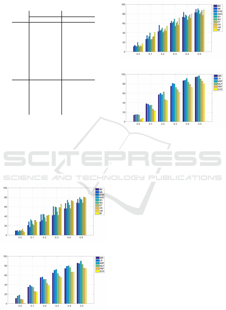
Table 3: Classification results (step=0.1).
Efron CCLRU
SR RMSE SR RMSE
BN 9.5 0.1516 11.4 0.1738
NB
9.5 0.2014 14.3 0.2221
SVM 10.5 0.209 12.4 0.2378
SMO
7.6 0.1731 11.4 0.152
IB1 10.5 0.209 20.0 0.2272
IB3
9.5 0.1675 13.3 0.1852
DT 9.5 0.1517 10.5 0.1734
OR 13.3 0.2056 11.4 0.239
J48
8.6 0.1911 9.5 0.2176
RF 6.7 0.1574 17.1 0.1741
IBR 11.4 0.3711 14.3 0.2932
LR
16.2 0.3728 15.2 0.2836
M5P 18.1 0.3416 15.2 0.2727
MLP
9.5 0.4188 14.3 0.3251
RBF 8.6 0.4402 4.8 0.3545
SVR
7.6 0.4677 7.6 0.376
number of images are classified in contiguous classes
which, in the case of step=0.1 is still an accurate clas-
sification. Figures 8, 9, 10, and 11 depict how the
success rate varies if we take into account the in-
stances that are classified in neighbouring classes. In
these figures, the x-axis shows the tolerance margins
whereas the y-axis shows the percentage of correct
classifications in that margin.
We can observe how in the CCLRU scale the
methods are able to classify more instances with
lower margin levels, while in the Efron scale only one
Figure 8: Evolution of the success rate in the classification
techniques (EFRON scale).
Figure 9: Evolution of the success rate in the regression
techniques (EFRON scale).
Figure 10: Evolution of the success rate in the classification
techniques (CCLRU scale).
Figure 11: Evolution of the success rate in the regression
techniques (CCLRU scale).
method achieves 90% of success rate for the maxi-
mum margin. The approaches that achieve the better
results are the regression techniques for both scales.
We can conclude that our system behaves like an
expert, as with a ±0.5 margin it is able to classify cor-
rectly 90% of the instances in the Efron scale. In the
CCLRU scale the results are better, as a ±0.4 margin
is enough to achieve more a 90% of success rate. We
think that this happens due to the nature of the proto-
types of each scale, since the Efron scale is made of
pictures whereas the CCLRU scale contains real eye
photographies. In consequence, gradings are easier
in the later scale, which is consistent with the system
behaviour.
4 CONCLUSIONS
The apparition of hyperemia in the bulbar conjunc-
tiva can be an early indicator of several pathologies,
such as conjunctivitis or dry eye syndrome. The pro-
cess that clinicians perform is tedious and subjective,
hence the importance of its automatisation in order to
provide objective and repeatable results. The present
work was focused in the transformation from the sev-
eral image features computed from a video frame of
the patient eye to a value in two given scales, Efron
and CCLRU. We performed severalexperimentscom-
paring the behaviour of classification and regression
techniques under different divisions of the data. Re-
ICAART 2016 - 8th International Conference on Agents and Artificial Intelligence
428

sults show that the system behaves like an expert, and
that regression methods perform better in both scales.
Future work will tackle the study of the evolution
of a patient, allowing us to measure the ratio of ap-
pearance of new vessels and other associated changes
that occur in the conjunctiva.
REFERENCES
Aha, D. W., Kibler, D., and Albert, M. K. (1991).
Instance-based learning algorithms. Machine learn-
ing, 6(1):37–66.
Baum, E. B. (1988). On the capabilities of multilayer per-
ceptrons. Journal of complexity, 4(3):193–215.
Breiman, L. (2001). Random forests. Machine learning,
45(1):5–32.
Buhmann, M. D. (2000). Radial basis functions. Acta Nu-
merica 2000, 9:1–38.
Canny, J. (1986). A computational approach to edge detec-
tion. Pattern Analysis and Machine Intelligence, IEEE
Transactions on, (6):679–698.
Chang, C.-C. and Lin, C.-J. (2011). LIBSVM: A library
for support vector machines. ACM Transactions on
Intelligent Systems and Technology, 2:27:1–27:27.
Cooper, G. F. and Herskovits, E. (1991). A bayesian
method for constructing bayesian belief networks
from databases. In Proceedings of the Seventh con-
ference on Uncertainty in Artificial Intelligence, pages
86–94. Morgan Kaufmann Publishers Inc.
Efron, N., Morgan, P. B., and Katsara, S. S. (2001). Valida-
tion of grading scales for contact lens complications.
Ophthalmic and Physiological Optics, 21(1):17–29.
Fieguth, P. and Simpson, T. (2002). Automated measure-
ment of bulbar redness. Investigative Ophthalmology
and Visual Science, 43(2):340–347.
Friedman, N., Geiger, D., and Goldszmidt, M. (1997).
Bayesian network classifiers. Machine learning, 29(2-
3):131–163.
Hall, M., Frank, E., Holmes, G., Pfahringer, B., Reutemann,
P., and Witten, I. H. (2009). The weka data min-
ing software: an update. ACM SIGKDD explorations
newsletter, 11(1):10–18.
Hastie, T., Tibshirani, R., et al. (1998). Classification by
pairwise coupling. The annals of statistics, 26(2):451–
471.
Holte, R. C. (1993). Very simple classification rules per-
form well on most commonly used datasets. Machine
learning, 11(1):63–90.
Jensen, F. V. (1996). An introduction to Bayesian networks,
volume 210. UCL press London.
John, G. H. and Langley, P. (1995). Estimating continuous
distributions in bayesian classifiers. In Proceedings
of the Eleventh conference on Uncertainty in artificial
intelligence, pages 338–345. Morgan Kaufmann Pub-
lishers Inc.
Keerthi, S. S., Shevade, S. K., Bhattacharyya, C., and
Murthy, K. R. K. (2001). Improvements to platt’s smo
algorithm for svm classifier design. Neural Computa-
tion, 13(3):637–649.
Kohavi, R. (1995). The power of decision tables. In Ma-
chine Learning: ECML-95, pages 174–189. Springer.
Papas, E. B. (2000). Key factors in the subjective and objec-
tive assessment of conjunctival erythema. Investiga-
tive Ophthalmology and Visual Science, 41(3):687–
691.
Platt, J. et al. (1999). Fast training of support vector ma-
chines using sequential minimal optimization. Ad-
vances in kernel methodssupport vector learning, 3.
Quinlan, J. R. (2014). C4. 5: programs for machine learn-
ing. Elsevier.
Quinlan, J. R. et al. (1992). Learning with continuous
classes. In 5th Australian joint conference on artificial
intelligence, volume 92, pages 343–348. Singapore.
Rodriguez, J. D., Johnston, P. R., Ousler III, G. W., Smith,
L. M., and Abelson, M. B. (2013). Automated grad-
ing system for evaluation of ocular redness associated
with dry eye. Clinical ophthalmology (Auckland, NZ),
7:1197.
Rolando, M. and Zierhut, M. (2001). The ocular surface
and tear film and their dysfunction in dry eye disease.
Survey of Ophthalmology, 45, Supplement 2(0):S203
– S210.
S´anchez, L., Barreira, N., Garc´ıa-Res´ua, C., and Yebra-
Pimentel, E. (2015a). Automatic selection of video
frames for hyperemia grading. Eurocast 2015, pages
165–166.
S´anchez, L., Barreira, N., Pena-Verdeal, H., and Yebra-
Pimentel, E. (2015b). A novel framework for hyper-
emia grading based on artificial neural networks. In
Advances in Computational Intelligence, pages 263–
275. Springer.
Schulze, M. M., Jones, D. A., and Simpson, T. L. (2007).
The development of validated bulbar redness grading
scales. Optometry & Vision Science, 84(10):976–983.
Smola, A. J. and Sch¨olkopf, B. (2004). A tutorial on
support vector regression. Statistics and computing,
14(3):199–222.
V´azquez, S. G., Barreira, N., Penedo, M. G., Pena-Seijo,
M., and G´omez-Ulla, F. (2013). Evaluation of SIRIUS
retinal vessel width measurement in REVIEW dataset.
In Proceedings of the 26th IEEE International Sym-
posium on Computer-Based Medical Systems, Porto,
Portugal, June 20-22, 2013, pages 71–76.
Wang, Y. and Witten, I. H. (1996). Induction of model trees
for predicting continuous classes.
Wolffsohn, J. S. and Purslow, C. (2003). Clinical monitor-
ing of ocular physiology using digital image analysis.
Contact Lens and Anterior Eye, 26(1):27–35.
Yoneda, T., Sumi, T., Takahashi, A., Hoshikawa, Y.,
Kobayashi, M., and Fukushima, A. (2012). Auto-
mated hyperemia analysis software: reliability and re-
producibility in healthy subjects. Japanese journal of
ophthalmology, 56(1):1–7.
Comparing Machine Learning Techniques in a Hyperemia Grading Framework
429
