
Determination of Parameters of Adaptive Law for the Control of an
Off-grid Power System
Konstantin Suslov
1
, Svetlana Solodusha
2
and Dmitry Gerasimov
1
1
Irkutsk National Research Technical Uuniversity, 83, Lermontov str., Irkutsk, Russia
2
Energy Systems Institute SB RAS, 130, Lermontov str., Irkutsk, Russia
Keywords: Smart Grid, Volterra Polynomials, Power Quality, Control Systems, Electric Power Systems, Distributed
Generation.
Abstract: The paper presents the results of a study of an off-grid electric power system that contains typical generation
and load devices. The aim of the study is to develop an algorithm for selecting the optimal parameters of
adaptive control law of the energy characteristics in the off-grid power system at the connection point of a
varied load. To this end a simulation experiment was carried out and its results were used to numerically
model the off-grid power system. The authors apply a known method of modelling the complex multi-
parametric systems represented by the Volterra integro-power series. Standard approaches to the
measurement of dynamic performance were applied to identify a transient response of the system.
1 INTRODUCTION
One of the main directions in power engineering is
the adoption of components applicable to the
implementation of a smart grid concept. The
considered system contains the main elements that
belong to the isolated (off-grid) systems. This makes
it possible to take into consideration the key features
of a change in the nature of generation when
changing the load parameters.
The input was represented by a symmetrical
change in a three-phase load of both active and
reactive components. The load changed in a step-
wise manner toward an increase (decrease) in the
load current. The parameters of the change in the
characteristics were taken into account at the
connection point of the varied load. The step-wise
change in the load occurred in the steady-state
operation of the system. Test inputs reached 50% of
the level of rated conditions. Since there is an
aperiodic component of three-phase currents in the
transient conditions a generalized positive-sequence
current phasor was measured. Also active and
reactive power flows at the connection point of the
varied load were taken into account.
2 STATEMENT OF THE
PROBLEM
The issues dealing with the selection of operating
conditions, network configuration (in terms of sites
for placement of generators), and reliability
assessment are considered by us in (Voropai, 2012;
Suslov, 2013).
The facilities to be considered as generators are:
gas turbine plants, wind turbines and solar panels.
Also, consideration is given to energy storage
devices, since the renewable energy output is
stochastic, their use is necessary to provide the
required reliability of electricity supply to
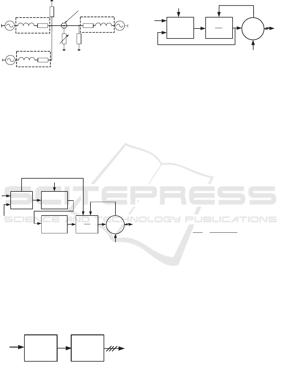
consumers of the off-grid systems. We consider an
isolated (off-grid) system scheme presented in Fig.
1. The experience gained in operating a gas turbine
plant reveals some serious problems when tuning the
automatic control loops, namely:
1. Lack of a comprehensive approach, because
power systems are considered separately from one
another.
2. The problem of obtaining common
algorithms for the power system control, which is
related to the complexity of traditional mathematical
tools.
Suslov, K., Solodusha, S. and Gerasimov, D.
Determination of Parameters of Adaptive Law for the Control of an Off-grid Power System.
In Proceedings of the 5th International Conference on Smart Cities and Green ICT Systems (SMARTGREENS 2016), pages 129-135
ISBN: 978-989-758-184-7
Copyright
c
2016 by SCITEPRESS – Science and Technology Publications, Lda. All rights reserved
129
Connection point
Z
2
Generator3
-
Gas turbine plant
Generator 1
-
Wind turbines
Generator 2
-
Solar panels
1
e
2
e
3
e
1
L
2
L
3
L
1
Z
3
Z
1
R
2
R
3
R
1
L
OAD
Z
2
L
OAD
Z
3
L
OAD
Z
Figure 1: A scheme of an isolated (off-grid) system
(
123
,,ee e
- electromotive force of different generators,
123
,,
Z
ZZ- internal impedance of the generators,
12
,
load load
ZZ-unchangeable fixed load of consumers,
3load
Z -variable load,).
We suggest the following approach to solve the
above problems. The electricity generating systems
are defined by the external structural input-output
schemes. The flow chart for the gas turbine plant is
presented in Figure 2.
i
P
P
F
Compressor
Combustion
chamber
Turbine
G
T
M
d
dt
E
U
,Uf
CC
M
CG
M
Generator
Figure 2: Flow chart for a single-shaft gas turbine plant
(U
E
-excitation voltage, U – voltage at the generator outlet,
f- network frequency, P- air pressure at the compressor
inlet, - angular velocity, P
i
- pressure at the compressor
outlet, F – fuel supplied to the combustion chamber, G-
gas flow rate, M
CC
- gas turbine shaft resistance torque
created by compressor, M
CG
- turbine shaft resistance
torque created by electric generator).
The flow chart for the solar panel is demonstrated in
Figure 3. The flow chart for the wind turbine plant
is shown in Figure 4.
I
nverter
1
U
S
E
2
,Uf
Solar
p
anel
Figure 3: Flow chart for solar panel (E
S
– solar energy, U
1
– voltage at the solar panel outlet).
E
U
,Uf
WT
M
V
b
CG
M
d
dt
Generator
Wind
Turbine
Figure 4: Flow chart for the wind turbine plant (V- wind
speed, b – attack angle, M
WT
- engine torque, created by
wind turbine).
Each of the generators has their specific features to
be taken into account in designing the automated
control system. For example, gas turbine plant
makes it possible to completely control input
parameters but has quite high inertia. Generation
from solar panels is deterministic due to the lack of
inertia.
Generation from wind power plants is a vivid
example of stochastic operation of generators. At the
same time, apart from the random change in the
input data such a generation is subject to inertia.
Figure 5 presents a subsystem of the wind
turbine module which is described by a system of
algebraic equations, where the input signals are
represented by wind speed V, attack angle of turbine
blade b, current coordinate of angular velocity
depending on the shaft resistance torque.
Inertia of the rotating parts in the wind turbine is
taken into account by the equation of dynamics
TC
M
M
d
dt J
, (1)
where
T
M
- turbine generator shaft torque,
C
M
-
resistive torque created by generator,
J
- total
inertia torque. Generally speaking, the analysis of
dynamic characteristics of wind power unit is based
on the methods using differential equations. Most of
the researches are devoted to the specification of
characteristics of individual components of wind
turbine (He, 2009; Li, 2011), specification of various
coefficients (Manyonge, 2012) or consideration of a
mechanical part of the turbine as an N-mass system
(Bhandari, 2014).
Traditionally, the theory of modelling the control
systems employs differential equations with constant
coefficients. These equations are obtained by
linearizing the nonlinear differential equations with
variable coefficients of the most typical operating
conditions of a certain system (Saadat, 2010, Ogata,
2010). This is explained by the presence of a
nondeterministic system with distributed parameters.
SMARTGREENS 2016 - 5th International Conference on Smart Cities and Green ICT Systems
130

V
R
z
T
3
1
10.035
0.08 1
i
z
zbb
i
z
i
p
eb
z
C
5.12
54.0
116
22.0
T
p
T
VSC
M
2
3
T
b
V
z
i
z
T
M
Figure 5: A subsystem of the wind turbine scheme ( C
m
-
torque coefficient,
- air density, V - wind speed, m/s; S -
blade-swept area, R - wind wheel radius, m,
2
2
P
P
С
VS
-
coefficient of wind energy use,
R
Z
V
– specific speed).
In practice, the initial data are known with some
error. In this case, as a rule, solutions to the inverse
problem turn out to be unstable with respect to an
error in the initial data. Therefore, to construct stable
methods we use the theory of ill-posed problems
(Kabanikhin, 2011).
Thus, all traditional methods are convenient for
the research and analysis of power system operation
but are hardly suitable for the implementation of an
adaptive response of a control system to the real-
time disturbances.
Also, such systems can be described by the
system of linear differential equations in the
neighbourhood of operation point (Salamanca, 2010,
Chenx, 2011) and by the system of differential
equations written in the normal Cauchy
form (steady-state) (Al-Jufout, 2010; Wang 2013,
2014)
We believe that the study can involve a known
mathematical modelling approach in which any
dynamic system is represented as a “black box”
(Fig.6). In the case, where the output y(t)
continuously depends on inputs x(t), the model of
nonlinear dynamic system can be represented by
Volterra integro-power series (Volterra, 1959).
()
x
t
()yt
Figure 6: The “input-output” system.
The studies show that wind power plant has the
greatest impact on the output value y(t). And the
larger the share of wind generation in the off-grid
system, the greater this impact is. The qualitative
character of this impact is demonstrated in Fig.7.
Here it was assumed that gas turbine plant and
photovoltaic cells share the rest of generation in
halves.
10
20 30 40 50 60
70 80
90
100
The share of wind power, %
1
Experimental outputs to the input disturbance, p.u
Figure 7: The qualitative character of the impact.
Thus, it is reasonable to consider the problem of the
off-grid system modeling on the example of a wind
power plant.
3 ABOUT A NEW APPROACH TO
THE MATHEMATICAL
DESCRIPTION OF THE WIND
POWER PLANT DYNAMICS
The Volterra integro-power series (Doyle, 2002;
Rugh, 1981; Venikov, 1982; Pupkov, 1976) are
widely used in mathematical modeling of complex
nonlinear dynamic systems. The nonlinear dynamic
systems and their properties are fully characterized
by multidimensional weight functions, i.e. Volterra
kernels. In this case the problem of constructing a
mathematical model of a nonlinear dynamic system
lies in the identification of Volterra kernels on the
basis of data obtained from the experimental
research into an input-output system (Giannakis,
2001).
In this research we employ an approach
(Apartsyn, 2013) based on the physically
implemented test inputs. The main distinction of this
approach lies in the fact that the initial problem is
reduced to solving special integral equations which
can be explicitly solved.
Determination of Parameters of Adaptive Law for the Control of an Off-grid Power System
131

In this research we have developed and
implemented new algorithms for the construction of
integral models represented by Volterra polynomials
with vector input
1
1
,..., 1
11 ,..., 2
1
00
( ) ... ( , ,..., ) ( )
nk
n
tt
n
N
ii n i k k
nii
k
yt K ts s x s ds
in the cases which are the most important for
applications,
2,3.N The research is a
continuation of (Suslov, 2015).
In (Solodusha, 2015) the authors show that the
problem of the Volterra kernels identification in the
quadratic Volterra polynomial
11 11
0
() (, ) ( ) +
t
quad
yt Ktsxsds
(2)
2
212
1
00
(, , ) ( )
tt
ii
i
K
ts s xs ds
,
[0, ]tT
can be solved by using only two integral equations
1
12 1 1 1
0
(, , ) (, )yt Ktsds
(3)
12
1
111 1
(, ) 3 (, ,0)Ktsds y t
12
3(,0, )yt
12 2
(, , )yt
112
1
111 111
0
7 (,) 5 (,)Ktsds Ktsds
,
112
1
111 111
0
(, ) (, )Ktsds Ktsds
(4)
11
2
21212
00
(, , )K t s s ds ds
11 2
1
2
21212
0
2(,,)K t s s ds ds
1212
11
2
21212 12
(, , ) (, , ).K t s s ds ds y t
The output
12
(, , )yt
in the right-hand side of
(3), (4) is a response of the reference dynamic
system (1) to the test inputs
12
,112
(() 2( ) ( ))xetetet
, (5)
where
12
,, [0,]tT
, ()et is the Heaviside
function:
0, 0,
()
1, 0.
t
et
t
In order to improve the accuracy of modelling we
will consider a modification of this algorithm for the
case of cubic Volterra polynomial. Let us consider a
combined cubic model
11 11
0
() (, ) ( ) +
t
cub
yt Ktsxsds
(6)
2
212
1
00
(, , ) ( )
tt
ii
i
K
ts s xsds
3
312 3
1
000
ˆ
(, , ) ( )
ttt
ii
i
K
sss xt sds
.
Using the above approach it is easy to see that the
condition of form (3) and outputs of the reference
dynamic system to the test inputs
12
(),
i
x
t
0,
i
1, 2,i
12
of form (5) make it
possible to completely identify the
kernels
123
ˆ
,,
K
KK
. For example, the restoration of
kernel
1
K is reduced to solving the integral
equation
1
111 1 1
0
(, ) (, )Ktsds ft
, (7)
where
1
2
3
11
3
12
11
3
11
3
22
(, )
(, )
(, )
ft
ft
ft
, (8)
11 1
1
(, ) (, ,0) (,0, )
2
iii
ft yt yt
As applied to the model
11 11
0
() (, ) ( ) +
t
cub
yt Ktsxsds
(9)
SMARTGREENS 2016 - 5th International Conference on Smart Cities and Green ICT Systems
132

2
212
1
00
ˆ
(, ) ( )
tt
ii
i
K
ss xt sds
3
312 3
1
000
ˆ
(, , ) ( )
ttt
ii
i
K
sss xt sds
we obtain, that for the unique restoration of
123
ˆˆ
,,
K
KK
it is sufficient to have outputs of a
dynamic system to the test inputs
12
(),
i
x
t
0,
i
1, 2,i
12
of form (4) and
condition
21 2 11
(, ) ( , )ft ft
.
In this case the problem of identification, for
example, of kernel
1
K
, can be reduced to equation
(9) with the right-hand side of (8), where
11 11
1
(, ) (, ,0) ( , ,0)
2
iii
f t yt yt
4 CASE STUDY
Based on the developed algorithms we constructed a
quadratic model of form (2) and a cubic model of
form (9). The identification involved the studied
system outputs (Fig.1) to the test inputs of form (5).
The input is considered to be a change in the
character of load power, and the outputs are
represented by the power system parameters. The
parameters were calculated for the connection point
demonstrated in Fig.1. A generalized vector of a
three-phase load current was used as a parameter.
The rest of the parameters were active and reactive
power at the connection point.
Figures 8-10 present the outputs of the reference
model (Fig. 1) to the input disturbances
( , ) 10( ( ) ( ))S t et et
,
where S - total load power.
These data were employed to restore transient
characteristics in the integral models. The accuracies
of quadratic and cubic models were compared in the
description of the studied off-grid electricity supply
system. The time of the transient process is Т=0.2
sec., which corresponds to real values of the
transient process time in the electric power systems.
The computational experiment demonstrated the
advantages of cubic model versus quadratic one.
Figure 11 illustrates the typical outputs of active
0.02 0.04 0.06 0.08 0.10 0.12 0.14 0.16 0.18 0.20
Time of the transition process, t sec
0
47
94
141
188
Power current, I A
Figure 8: Values of power current at the connection point.
0.02 0.04 0.06 0.08 0.10 0.12 0.14 0.16 0.18 0.20
Time of the transition process, t sec
2
0
4
6
8
10
12
Active power, P kW
Figure 9: Values of active power at the connection point.
Time of the transition process, t sec
-0,45
Reactive power, Q kVAr
0.02
0.04
0.06 0.08 0.10 0.12 0.14
0.16
0.18 0.200
-0,95
-1,45
-1,95
-2,45
-2,95
-3,45
-3,95
-4,45
-4,95
Figure 10: Values of reactive power at the connection
point.
power at load shedding. They were obtained using
quadratic and cubic models. Curve 1 denotes a
steady-state value; curves 2 and 3 were obtained
using quadratic and cubic models, respectively;
curve 4 stands for an accurate value obtained using
the reference model.
Curve 3 illustrates an effect of the inclusion of
additional terms, i.e. an essential nonlinear character
of the studied output.
Determination of Parameters of Adaptive Law for the Control of an Off-grid Power System
133

0,05 0,10
0,15
0,20
Time of the transition process. t sec
1
2
3
4
Figure 11: System outputs.
5 PARAMETER OPTIMIZATION
IN TEST INPUTS (5)
Let in (5)
0
. The extreme problem of choosing
*
for some standard mathematical model is
formulated in (Apartsyn, 2013). Let us consider by
analogy the optimal (in some or other sense) choice
of
in (4) to identify the kernels
1
K
and
2
K
in
(1).
We choose some
from a range
],[ BB
. Take
the set
(,) { ()XBT x t
( ( ) ( )),et et
[,],0 }
B
BtT
(10)
as a class of the admissible inputs )(tx .
As the system response value at the end of the
considered transient process (
Tt
) plays an
important role in applications, the criterion of model
accuracy has the form
,
[0, ]
() ( , )
max | ( , ) ( , ) | min
et quad
B
xtXBT
yT y T
,
where
,
(, )
quad
yT
is response (2) to the input
()St
(10). Actually, the difference
,
(, ) (, )
et quad
yT y T
is some function of the
parameters
,,
.
Then
),,(maxminarg*
],[
],0[
],0[
N
BB
T
B
, (11)
where
,
(, , ) (, ) (, )
et quad
NyTyT
.
We present the results of mathematical modeling
that were obtained using the software (Gerasimov,
2015).
The set
),( TBX
of such inputs as
()St
;
],0[ B
,
0
50% ;
B
S
0.2T
sec. was taken as
admissible. The calculations showed that
T
max
,
2
,
max
B
B
.
The calculations demonstrate that the value
*
0.9B
, at
0
50%
B
S
.
The plot of the function
|),*,(|
N
with
0
50%
B
S
,
0.2T
sec. is given in Fig. 12.
0,05
0,10 0,15
0,20
*
N
Figure 12: The plot of the function
|),*,(|
N
.
Analysis of the results obtained for the reference
model (1) enables us to recommend that for the
identification of Volterra kernels the parameter
of test inputs (5) be chosen in the range
0.75 0.9
B
B
.
6 CONCLUSIONS
Consideration is given to a model of an off-grid
system represented as a quadratic segment of the
Volterra integro-power series on the basis of a
reference model. The reference model is represented
by an isolated electric power system, which contains
several electricity sources, storage systems, and the
shunt- and series-connected devices (active
elements) that allow an on-line change in the energy
parameters of the system. A system of algorithms is
developed to control the most characteristic
operating conditions of the power system, which can
be used for on-line technical implementation.
SMARTGREENS 2016 - 5th International Conference on Smart Cities and Green ICT Systems
134

ACKNOWLEDGEMENTS
The research was supported by the grant of the
RFBR No. 15–01–01425–a.
REFERENCES
Voropai, N.I., Suslov, K.V., Sokolnikova, T.V.,
Styczynski, Z.A., Lombardi, P., 2012. Development of
power supply to isolated territories in Russia on the
bases of microgrid concept, in Proc. 2012 IEEE Power
and Energy Society General Meeting.
Suslov, K.V., 2013. Development of isolated systems in
Russia, in Proc. 2013 IEEE PowerTech.
He, Z., Xu, J., Xiaoyu, W., 2009. The dynamic
characteristics numerical simulation of the wind
turbine generators tower based on the turbulence
model, in Proc. 2009 4th IEEE Conference on
Industrial Electronics and Applications (ICIEA).
Li, J., Chen, J., Chen, X., 2011. Dynamic Characteristics
Analysis of the Offshore Wind Turbine Blades,
Journal Marine Sci., vol.10, pp. 82-87.
Manyonge, A.W., Ochieng, R.M., Onyango, F.N.,
Shichikha, J.M., 2012. Mathematical Modelling of
Wind Turbine in a Wind Energy Conversion System:
Power Coefficient Analysis, Applied Mathematical
Sciences, vol.6. No. 91, pp. 4527-4536.
Bhandari, B., Poudel, S., Lee, K., Ahn, S.,2014.
Mathematical Modelling of Hybrid Renewable Energy
System: A Review on Small Hydro-Solar-Wind Power
Generation, International Journal of Precision
Engineering and Manufacturing-Green Technology,
vol.1, No. 2, pp.157-173.
Saadat, H., 2010. Power System Analysis. 2rd Edition,
New York: The McGraw-Hill Primis, pp. 528-562.
Ogata, K., 2010. Modern Control Systems, 5th Edition,
United States: Prentice Hall Publications, pp. 669-674.
Kabanikhin, S.I., 2011. Inverse and Ill-posed problems.
Theory and applications, Germany: De Gruyter.
Salamanca, J.M., Rodriguez, O.O., 2010. LMI's control
using a system of three power generators based on
differential algebraic model, in Proc 2010 IEEE
ANDESCON.
Chenx, L., Jiang, J.N., Choon, Y.T., Runolfsson, T., 2011.
A study on the impact of control on PV curve
associated with doubly fed induction generators, in
Proc 2011 IEEE PES Power Systems Conference and
Exposition (PSCE).
Al-Jufout, S.A., 2010. Differential-algebraic model of ring
electric power systems for simulation of both transient
and steady-state conditions, in Proc. 2010 15th IEEE
MELECON.
Wang, X., Chiang, H.D., 2014. Quasi steady-state model
for power system stability: Limitations, analysis and a
remedy, in Proc 2014 Power Systems Computation
Conference (PSCC).
Wang, X. Z., Chiang, H. D., 2013. Analytical Studies of
Quasi Steady-State Model in Power System Long-
term Stability Analysis, IEEE Transactions on
Circuits and Systems I: Regular Papers.
Volterra, V., 1959. A Theory of Functionals, Integral and
Integro-Differential Equations, New York: Dover
Publ.
Doyle III, F., Pearson, R., Ogunnaike, B., 2002.
Identification and Control Using Volterra Models,
Springer-Verlag.
Rugh, W.J., 1981. Nonlinear System Theory: The
Volterra/Wiener Approach, Johns Hopkins University
Press, Baltimore.
Venikov, V.A., Sukhanov, O.A., 1982. Cybernetic models
of electric power systems, Moscow: Energoizdat, (in
Russian).
Pupkov, K.A., Kapalin, V.I., Yushenko, A.S., 1976.
Functional Series in the Theory of Non-Linear
Systems, Moscow: Nauka (in Russian).
Giannakis, G.B., Serpedin, E., 2001. A bibliography on
nonlinear system identification and its applications in
signal processing, communications and biomedical
engineering, Signal Processing — EURASIP, vol. 81,
No. 3, pp. 533-580.
Apartsyn, A.S., Solodusha, S.V., Spiryaev, V.A., 2013.
Modeling of Nonlinear Dynamic Systems with
Volterra Polynomials: Elements of Theory and
Applications, IJEOE, vol. 2, No. 4, pp. 16-43.
Suslov K.V., Gerasimov D.O., Solodusha S.V., 2015.
Smart Grid: Algorithms for Control of Active-
Adaptive Network Components, PowerTech.
Solodusha, S.V., Suslov, K.V., Gerasimov, D.O., 2015. A
New Algorithm for Construction of Quadratic Volterra
Model for a Non-Stationary Dynamic System, IFAC-
Papers Online, vol. 48, No. 11, pp. 992-997.
Gerasimov, D.O., Suslov, K.V. A simulation model of a
horizontal-axis wind turbine. State registration
certificate for the computer software No. 2016610203,
11.01.2016 (in Russian).
Determination of Parameters of Adaptive Law for the Control of an Off-grid Power System
135
