HMM-based Transient and Steady-state Current Signals Modeling for

Electrical Appliances Identiﬁcation

Mohamed Nait-Meziane

, Abdenour Hacine-Gharbi

, Philippe Ravier

, Guy Lamarque

Jean-Charles Le Bunetel

and Yves Raingeaud

PRISME Laboratory, University of Orl

eans, 12 Rue de Blois, 45067 Orl

eans, France

LMSE Laboratory, University of Bordj Bou Arr

eridj, Elanasser, 34030 Bordj Bou Arr

eridj, Algeria

GREMAN Laboratory, UMR 7347 CNRS - University of Tours, 20 Avenue Monge, 37200 Tours, France

Keywords:

Electrical Appliances Identiﬁcation, Energy Disaggregation, Harmonic Analysis, Hidden Markov Mod-

els (HMM), Non-Intrusive Load Monitoring (NILM), Parameter Relevance, Short-Time Fourier Se-

ries (STFS), Smart Grids, Transient and Steady-state Electrical Signal Analysis.

Abstract:

The electrical appliances identiﬁcation problem is gaining a rapidly growing interest these past few years due

to the recent need of this information in the new smart grid conﬁguration. In this work, we propose to construct

an appliance identiﬁcation system based on the use of Hidden Markov Models (HMM) to model transient and

steady-state electrical current signals. For this purpose, we investigate the usefulness of different choices for

the proposed identiﬁcation system such as: the use of the transient and the steady-state current signals, the use

of even and odd-order harmonics as features, and the optimal number of features to take into account. This

work also discusses the choice of the Short-Time Fourier Series (STFS) coefﬁcients as adapted features for

the representation of transient and steady-state current signals.

1 INTRODUCTION

The way power grids work to provide the needed elec-

trical energy has changed a lot in the last few years.

Classically, in the power grid, the energy goes only

one way, i.e. from the power stations (usually ther-

mal) to the consumers. With the advent of the idea of

exploiting renewable energy resources (wind power,

solar power, hydropower, etc.) the ﬂow of energy in

the power grid can no longer go only one way. A con-

sumer having a wind turbine, solar cells, or other

renewable-based energy generation systems becomes

also an energy producer and this gives rise to a decen-

tralized energy production. Also, in this new conﬁg-

uration, the energy production is no longer based on

one energy source (thermal) but it can be generated

using different, eventually renewable, energy sources.

These new mutations created the need for an upgrade

to the power grid and the result is what we call a smart

grid.

As deﬁned in (Gellings, 2009): “a smart grid is the

use of sensors, communications, computational abil-

ity and control in some form to enhance the overall

functionality of the electric power delivery system.”

Adding these features to a power grid allows a bet-

ter monitoring and a continuous supervision of the

energy ﬂow. The energy sensors (or energy meters)

along with their communication and computational

capabilities are the basic building block of a smart

grid. An energy meter allows the access to the energy

consumption information of the appliance or group of

appliances it measures.

The importance of energy metering and detailed

electrical consumption information has been dis-

cussed in several previous works (Fischer, 2008)

(Darby, 2006) (Darby, 2010) (Hancke et al., 2012).

The impact of this information on the consumer be-

havior has been studied in (Chakravarty and Gupta,

2013) where the results showed that on average the

consumers that used a solution that allowed the break

down of the energy consumption consumed on aver-

age 14% less energy than the consumers that did not

use it. According to (Carrie Armel et al., 2013), the

beneﬁts of appliance-level electrical consumption in-

formation over global consumption fall into three cat-

egories: (1) beneﬁts to the consumer through possi-

ble energy savings thanks to the consumption feed-

back, (2) research and development beneﬁts since the

feedback allows the understanding of appliance en-

ergy consumption proﬁles and then redesigning ap-

670

Nait-Meziane, M., Hacine-Gharbi, A., Ravier, P., Lamarque, G., Bunetel, J-C. and Raingeaud, Y.

HMM-based Transient and Steady-state Current Signals Modeling for Electrical Appliances Identiﬁcation.

DOI: 10.5220/0005759506700677

In Proceedings of the 5th International Conference on Pattern Recognition Applications and Methods (ICPRAM 2016), pages 670-677

ISBN: 978-989-758-173-1

pliances for energy efﬁciency, and (3) utility and pol-

icy beneﬁts such as allowing for improved load fore-

casting (Feinberg and Genethliou, 2005) and energy

demand prediction which is very important when it

comes to decision making and taking economically

reliable actions either by utilities or governments.

2 GENERAL BACKGROUND FOR

ELECTRICAL APPLIANCES

IDENTIFICATION

To break down the global energy consumption into

its different constituent parts (for example, the whole

home energy consumption into the appliance-level

energy consumption) three approaches can be consid-

ered: intrusive, semi-intrusive, and non-intrusive ap-

proaches.

Intrusive Load Monitoring (ILM) approaches are

based on the use of distributed sensing meters to sup-

port control, monitor and intervention of such de-

vices (Burbano Acu

na, 2015). As stated by (Parson,

2012) different forms of ILM can be found:

• Electrical sub-metering: one energy meter is used

for each appliance

• Smart appliances: the appliances have communi-

cating chips that allows them to self-report their

energy consumption to a central unit

• Electrical probing: transmitting an electrical sig-

nal into the households mains circuit and analyz-

ing the return signal

The ILM do not seem to be viable solutions since

they assume the installation of different energy meters

in different household locations which is not easy to

do and most of the time costly. Semi-Intrusive Load

Monitoring (SILM) is somehow a relaxed version of

the ILM, where instead of using energy meters one

per appliance, we use one energy meter to measure a

group of appliances (Tang et al., 2014). SILM share

the same drawbacks of the ILM but with less intru-

sion. Very little information can be found, in the lit-

erature, on SILM and this may be because they are

usually confused with ILM approaches.

Non-Intrusive Load Monitoring (NILM) is a ﬁeld

where the main concern is to break down an ag-

gregated energy consumption into its different con-

stituent parts in a non-intrusive way using only one

energy meter. For example, instead of introducing

different energy meters put all around the household

we only put one energy meter at the main breaker

panel level. The work on this ﬁeld started with Hart

in the late 1980s (Hart, 1989) (Hart, 1992) where he

proposed to use the (real) power consumption varia-

tion to identify household appliances. Even though

some other work was done in this ﬁeld after Hart

between the early 1990s and the late 2000s (Sul-

tanem, 1991) (Leeb et al., 1995) (Cole and Al-

bicki, 1998) (Drenker and Kader, 1999) (Chan et al.,

2000) (Baranski and Voss, 2003) (Laughman et al.,

2003) (Ting et al., 2005) (Patel et al., 2007) (Chang

et al., 2008) it was not until around ﬁve years ago

that this ﬁeld started to gain a rapidly growing inter-

est. A state of the art for the NILM techniques can be

found in (Najmeddine et al., 2008) (Du et al., 2010)

and (Zeifman and Roth, 2011). In (Carrie Armel

et al., 2013) the authors gave a table that summa-

rizes some of the works done in the NILM ﬁeld up

to 2012. They organized them in a chronological or-

der and gave some details on the used methods, data

types, appliance types, data frequency, and other in-

teresting characteristics.

In this study we propose the use of Hidden

Markov Models (HMM) for transient electrical sig-

nals modeling and classiﬁcation. The obtained fea-

tures are to be used eventually as a complementary

information that helps a NILM system identify home

appliances. Previous work on NILM using HMM was

done by (Zia et al., 2011) (Beckel et al., 2012) (Par-

son, 2012) and more recently by (Ridi and Hen-

nebert, 2014) and (Parson et al., 2014). In these stud-

ies, the authors applied their proposed approaches on

low-frequency sampled signals (for example, (Beckel

et al., 2012) used the REDD dataset

with 1 Hz

sampling frequency signals and (Ridi and Hennebert,

2014) used the ACS-F1 dataset

that has 10 Hz sam-

pling frequency signals). In our study, we propose

the use of HMM on high-frequency sampled signals

and we use for this purpose the recently released

PLAID dataset (PLAID, 2015). It is worth mention-

ing that the lack of a proper database that is informa-

tive, diverse, and scalable (Lai et al., 2012) of high-

frequency sampled electrical signals for appliances

hindered a lot the development of high-frequency

NILM. This was one of the concerns that have been

discussed by the NILM community during the 2nd

European NILM workshop (July, 2015) held in Lon-

don

In the literature, and to the best of our knowl-

edge, the authors of (Thiruvaran et al., 2013) are the

only ones, to date, that have done a study on high-

frequency sampled signals (10 kHz) using HMM.

In (Thiruvaran et al., 2013) the authors proposed to

http://redd.csail.mit.edu/

http://www.wattict.com/web/index.php/databases/acs-

http://www.nilm.eu/

HMM-based Transient and Steady-state Current Signals Modeling for Electrical Appliances Identiﬁcation

671

use the Short-Time Fourier Transform (STFT) and

Wavelet Tranform (WT) coefﬁcients as features for

their identiﬁcation system and as a dataset they col-

lected measurements of current and voltage wave-

forms for four different appliances (a ﬂuorescent

lamp, an incandescent lamp, a computer monitor, and

a motor). To acquire the waveforms, these four ap-

pliances were used to form switching-on sequences

(24 possible sequence in total). For example, as a se-

quence we can imagine: the ﬂuorescent lamp is ﬁrst

turned-on, then the incandescent lamp, then the com-

puter monitor and then the motor. Finally, they an-

nounced accuracies of 97.9% when using the STFT

features and 93.75% when using the WT features. In

our study, we propose to consider not only the tran-

sient but also the steady-state and we quantify the use-

fulness of the transient part over the steady-state part

for appliance recognition. Also, the accuracies ob-

tained in (Thiruvaran et al., 2013) can not quantify the

real recognition accuracy of the HMM-based system

due to the small size of the used dataset. This is why

the use of the PLAID dataset should allow more reli-

able results. Along with this, we propose in our study

the evaluation of the harmonic-order on the recogni-

tion accuracy of the proposed HMM-based system

instead of just taking into account all the harmon-

ics. Another difference compared to the work done

in (Thiruvaran et al., 2013) is that the PLAID dataset

signals are electrical signals of individual appliances.

That means that each signal was acquired with only

one appliance operating alone. Analyzing such sig-

nals should allow the determination of intrinsic high-

frequency characteristic features for the different ap-

pliances that can be used afterwards as a complemen-

tary information in a larger recognition system with

data fusion capabilities.

3 HARMONIC ANALYSIS

There are different ways to analyze the harmonic con-

tents of a signal. The most known method is the use of

the Fourier Transform (FT). For a discrete-time signal

s[n] we deﬁne the Discrete Fourier Transform (DFT)

as follows (Mallat, 1999):

S [k] =

L−1

∑

n=0

s[n]exp



− j2πkn



, k = 0, . .., L − 1

(1)

where L is the length of s[n] in samples. The com-

putation of the harmonic content of s[n] using Equa-

tion 1 starts to become heavier as L becomes bigger

and bigger even when using fast algorithms like the

Fast Fourier Transform (FFT), especially, when the

dataset is big and a lot of signals have to be analyzed.

Since the electrical current signals are periodic (the

steady-state signals), we propose to exploit this char-

acteristic to improve the computational time using the

Fourier Series (FS) decomposition instead of the FT.

The FS are particular instances of the FT for Dirac

sums (Mallat, 1999). This means that to get the FT

of a periodic signal we only have to compute its FS

coefﬁcients. For the periodic signal s[n], the Discrete

FS (DFS) decomposition is:

s[n] =

N−1

∑

k=0

exp



j2πkn



, (2)

where N is the period of s[n] in samples and

N−1

∑

n=0

s[n]exp



− j2πkn



, k = 0, . .., N − 1

(3)

are the DFS coefﬁcients of s[n]. Even though, Equa-

tions 1 and 3 look similar (up to a factor), the main

difference is the number of samples over which the

sum is computed. By summing over the signal pe-

riod N (usually < L) instead of over the whole signal

length we gain in computational time.

The DFS coefﬁcients C

, k = 1, ..., N − 1

(Equation 3) correspond to the fundamental fre-

quency of the periodic signal (k = 1) and its har-

monics. For the steady-state electrical current signals

these frequencies appear to represent most, if not all,

of the information contained in the signal. Hence, this

is another reason that justiﬁes the use of the DFS in-

stead of the DFT.

For transient electrical current signals, however,

the periodicity property is lost and strictly speaking

we are not allowed to use Equations 2 and 3. Nev-

ertheless, we think that even for the transient signals,

the important of the signal information is contained

around the fundamental frequency and its harmonics.

That is why we chose to represent the transient signals

also using the DFS coefﬁcients.

Since our approach is based on dividing the elec-

trical current signals (transient and steady-state) into

overlapping windows and computing the DFS on each

window, the obtained coefﬁcients can be called Short-

Time Fourier Series (STFS) coefﬁcients. Hence, for

the remainder of the paper we will use the notation

STFS instead of DFS. Each STFS coefﬁcients’ vec-

tor (computed on a window) is called an observation.

Thus, each waveform (an electrical current signal) is

represented by a sequence of vectors considered as a

sequence of observations for the HMM-based classi-

ﬁcation.

ICPRAM 2016 - International Conference on Pattern Recognition Applications and Methods

672

4 EXPERIMENTAL RESULTS

AND DISCUSSION

The appliance identiﬁcation system is mainly based

on three things: a dataset, a feature extraction (even-

tually feature selection) algorithm, and a classiﬁer.

As dataset we chose the PLAID dataset for which

we give a brief description in the next sub-section.

This dataset contains current and voltage waveforms

(sometimes instantaneous power) of different appli-

ances. For our study, we have decided to only use

the current waveforms as an appliance signature for

two main reasons. The ﬁrst one is that the voltage

waveform does not change much for the different ap-

pliances and hence does not add much information to

the identiﬁcation system. Actually, from a theoretical

point of view, the voltage waveform is not supposed

to change. We expect the voltage waveform to always

be a sine wave with a ﬁxed frequency equal to the

power line frequency of 50 or 60 Hz (depending on

the considered country) and a ﬁxed root-mean-square

(rms) voltage. Even though this is not a hundred per-

cent true (since there are always ﬂuctuations in the

power grid characteristics) we can assume to a certain

degree that it is the case in practice. The second rea-

son is that we found on the dataset a lot of voltage

waveforms that are incorrectly calibrated (i.e. having

incorrect amplitude values that diverge a lot from the

standard rms value of the grid voltage).

The used feature extraction algorithm is based on

the STFS already discussed in section 3 and the con-

sidered features are the magnitudes of the STFS co-

efﬁcients. For the classiﬁer we chose to use Hid-

den Markov Models (HMM) for their capabilities to

model dynamic time variations of signals.

An HMM is a ﬁnite state machine which changes

state once every time unit (the value of the time unit

depends on the observed phenomenon). Each time t

that a state j is entered, an observation vector o

generated from a probability density b

). The tran-

sition from state i to state j is also probabilistic and is

governed by the discrete probability a

i j

. The emission

likelihood b

for state j and observation o

at time t is

done by a Gaussian Mixture Model (GMM) (Hacine-

Gharbi et al., 2012):

) =

∑

m=1

N (o

;µ

,Σ

), (4)

where N (o; µ,Σ) is the value in o of a multivariate

Gaussian with mean µ

µ and covariance Σ. M Gaussians

are used in a mixture, each weighed by c

The classiﬁer is based on modeling each appliance

type by an HMM using the Hidden Markov Model

Toolkit (HTK) library (Young et al., 2009). The train-

ing is done in several steps by applying the embed-

ded Baum–Welch reestimation (HEREST command).

For the identiﬁcation step we used the Viterbi algo-

rithm (HVITE command). More details on the al-

gorithms used for training and identiﬁcation can be

found in (Young et al., 2009). For our identiﬁcation

system, we chose to model each appliance type us-

ing 3 states, and each state using 3 Gaussian mix-

tures. Each waveform was subdivided into overlap-

ping windows and from each window N features can

be extracted (even though in practice we only choose

a reduced number to work with, see the end of sub-

section 4.4). The window size was ﬁxed to 16.7 msec

(500 samples at 30 kHz frequency) that corresponds

to the 60 Hz cycle-time and the overlapping to 50%

of the window size.

The identiﬁcation results are evaluated using the

Classiﬁcation Rate (CR) deﬁned as:

CR(%) =

T − M

× 100, (5)

where T is the total number of tested waveforms

(each one representing an appliance) given to the in-

put of the classiﬁer and M is the number of misclassi-

ﬁed tested waveforms.

4.1 Summary of the PLAID Dataset

The Plug Load Appliance Identiﬁcation Dataset

(PLAID) is a public dataset of electric signatures.

These signatures are current and voltage measure-

ments taken during the summer of 2013 in Pittsburgh,

Pennsylvania, USA, from 55 households. This dataset

contains 11 appliance types and for each appliance

from three to six instances (the dataset contains a to-

tal of 1074 instances). Each signature of the dataset

is a few-second-long signal containing the turn-on

transient (when available, since for some appliances

like the “Fridge” for example, which is usually work-

ing all the time, the turn-on transient is not always

present) and a portion of the steady-state part (that

corresponds to the steady consumption phase). These

signals are sampled at a 30 kHz rate. Table 1 summa-

rizes the appliances found on the dataset: the differ-

ent appliance types and the number of instances for

each type. For more details on the dataset please refer

to (Gao et al., 2014). Finally, it is worth pointing out

that the values of the number of instances we found

in the dataset for each appliance type were most of

the time different than the ones given in (Gao et al.,

2014). The total number of instances in the dataset is

also different. This might be due to an update of the

dataset after the publication of the paper (Gao et al.,

2014).

HMM-based Transient and Steady-state Current Signals Modeling for Electrical Appliances Identiﬁcation

673

Table 1: Summary of the appliances found on the PLAID

dataset.

Appliance type Number of instances

Air Conditioner 66

Compact Fluorescent

Lamp

175

Fan 115

Fridge 38

Hairdryer 156

Heater 35

Incandescent Light

Bulb

114

Laptop 172

Microwave 139

Vacuum cleaner 38

Washing Machine 26

Total 1074

4.2 PLAID Dataset Subdivision for

Training and Tests

In this work, the dataset is divided into a training set

that allows the learning of appliances HMM mod-

els and a test set for the performance evaluation of

the identiﬁcation system. It is considered that all the

houses (55 in total) have examples in the training and

in the test sets. In order to study the effect of the num-

ber of waveform versions belonging to training and

test sets, we proposed four subdivisions. In the ﬁrst

one, we take for each house, at most one version of the

reference signal corresponding to a particular appli-

ance and the other versions are kept for testing. This

subdivision gives us 230 training waveforms and 844

test waveforms. The other subdivisions are obtained

by changing the maximum number of waveform ver-

sions to put in the training set from 2 to 4. Thus, we

got the four subdivisions shown in Table 2, where sbi

Table 2: Different tested subdivisions of the dataset

sb # sb1 sb2 sb3 sb4

NTR 230 441 648 848

NTEST 844 633 426 226

indicates the subdivision with “i” waveform versions

in the training set. NTR is the number of the consid-

ered training waveforms and NTEST is the number

of the considered test waveforms. For the following

sub-sections, the results are given for each one of the

above mentioned subdivisions.

4.3 Transient vs. Steady-state Electrical

Signals Usefulness for Appliance

Identiﬁcation

The goal of the experiment done in this sub-section is

to study the usefulness of the transient and the steady-

state parts of the electrical current signals for the iden-

tiﬁcation task of the different appliances. This ex-

periment required us to segment the PLAID dataset

waveforms each into a transient part and a steady-

state part. This segmentation was done by character-

izing the transient part as the one with the large energy

variation compared to the steady-state part. For the

performance evaluation, the classiﬁcation rate CR us-

ing the transient part (TP), steady-state part (SSP) and

the overall part (OP) was computed. This evaluation

takes into account the different dataset subdivisions

mentioned in sub-section 4.2. Note that in this exper-

iment, we only used 10 STFS coefﬁcients. Table 3

gives the CR for each subdivision sbi each time con-

sidering a different waveform part (OP, TP and SSP).

Table 3: Transient vs. Steady-state CR evaluation.

sb # sb1 sb2 sb3 sb4

CR (%), OP 86.02 87.36 87.56 88.50

CR (%), TP 88.98 91.15 90.85 92.48

CR (%), SSP 86.61 88.94 86.62 88.50

From these results, we can say that the use of the

transient part is the one that gives the best CR. More-

over, the results show that the computational time

when using only the transient part is much lower com-

pared to the others. For example, in the case of sb2,

the running test time was 218 seconds for TP, 418 sec-

onds for SSP, and 436 seconds for OP. The hardware

used for the experiment is a computer with an Intel

Core i5 processor and 4 GB of RAM memory.

Thereby, the use of the transient should allow the

construction of an appliance identiﬁcation system that

is fast and accurate which justiﬁes its usefulness for

the appliance identiﬁcation task. In order to improve

the identiﬁcation, we studied further the harmonic

analysis by taking into account the harmonic order

(even or odd) and the optimal number of STFS co-

efﬁcients to choose. The details are given in the next

sub-sections.

4.4 Even vs. Odd Harmonic Order for

Appliance Identiﬁcation

The experiment presented in this sub-section allows

the study of the harmonic order (even or odd or-

der) relevance for the appliance identiﬁcation task.

ICPRAM 2016 - International Conference on Pattern Recognition Applications and Methods

674

This experiment is similar to the one done in sub-

section 4.3 but we only consider the transient part,

following the results of sub-section 4.3. For the per-

formance evaluation, we compared the identiﬁcation

system CR when using even harmonics only, odd har-

monics only, and when using both. For each one of

these conﬁgurations, we used the corresponding ﬁrst

5 STFS coefﬁcients as features (i.e, ﬁrst 5 even har-

monics, ﬁrst 5 odd harmonics, and ﬁrst 5 harmon-

ics independently of the order, respectively). Table 4

gives the obtained CR for each tested conﬁguration.

From Table 4, we can deduce the following conclu-

Table 4: Even vs. Odd CR evaluation.

sb #

sb1 sb2 sb3 sb4

CR (%),

(even+odd)

88.98 91.15 90.85 92.48

CR (%),

even

63.63 64.45 64.79 63.27

CR (%),

odd

90.05 89.57 89.44 90.71

sions:

• The odd-order harmonics give the best perfor-

mance results no matter the considered subdivi-

sion w.r.t. the even-order harmonics

• The even-order harmonics give the worst perfor-

mance results

• Adding the even-order harmonics to the odd-order

harmonics feature vector does not seem to im-

prove a lot the CR

To conclude, the coefﬁcients of the fundamental and

its odd harmonics are the most useful for the appli-

ance identiﬁcation task. This can be explained by the

half-wave symmetry usually found in electrical sig-

nals (i.e. for a periodic signal g(t) with period T , we

have g(t) = −g(t ±T /2)) (Nait Meziane et al., 2015).

This half-wave symmetry causes the even order coef-

ﬁcients to have null values.

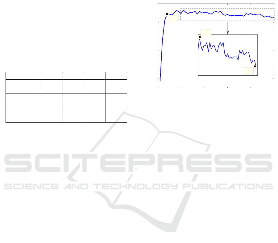
4.5 Optimal Number of Harmonics for

Appliance Identiﬁcation

A very important parameter to take into account is the

optimal number (the smallest) of STFS coefﬁcients to

consider in order to guarantee the best CR. To get

an insight on what this optimal number is, we eval-

uated the identiﬁcation system using various feature

vector (STFS coefﬁcients number) sizes. We only

considered the odd harmonics coefﬁcients from 1 to

50. Figure 1 gives the obtained results. This ﬁgure

shows the CR function of the odd harmonics number

taken into account for the identiﬁcation. The results

show that no signiﬁcant improvement is noticed when

taking more than 4 odd harmonics.

0 10 20 30 40 50

X: 4

Y: 89.44

Number of considered odd harmonics

CR (%)

10 15 20 25 30 35 40 45 50

X: 11

Y: 91.55

Number of considered odd harmonics

X: 49

Y: 87.32

X: 11

Y: 91.55

CR (%)

Figure 1: CR function of the considered odd harmonics

number.

Moreover, after reaching a peak value (when tak-

ing 11 odd harmonics) and after ﬂuctuating around

a more or less stable value (when taking up to 27

odd harmonics) that is smaller than the peak value,

the CR starts decreasing (see the zoom on Figure 1)

as we start taking more and more coefﬁcients. This

phenomenon is very known in pattern recognition and

is called the curse of dimensionality or peaking phe-

nomenon (Jain et al., 2000). The dimension of the

feature vector depends on the dimension of the dataset

used. To avoid this problem, and as a rule of thumb,

we usually say that the number of training data points

should be an exponential function of the feature vec-

tor dimension (Jain et al., 2000).

5 CONCLUSIONS

In this paper, we have discussed the use of HMM

models to solve the electrical appliance identiﬁcation

problem based on high-frequency sampled signals.

We have evaluated the usefulness of different choices

for the identiﬁcation system (the use of transient vs.

steady-state signals, even vs. odd-order harmonics as

features, and the optimal feature vector size). We

conclude from this study that the combined use of

the transient part of the electrical current signals with

only a few odd-order harmonics allows to construct an

appliance identiﬁcation system that is accurate, fast,

and less complex in terms of memory occupancy and

computations. In future work, and for more complete

results, the use and comparison of different types of

classiﬁers and different features may be considered.

HMM-based Transient and Steady-state Current Signals Modeling for Electrical Appliances Identiﬁcation

675

ACKNOWLEDGEMENTS

The authors would like to thank the R

egion Centre-

Val de Loire (France) for their ﬁnancial support of the

project MDE-MAC3 (Contract n

◦

2012 00073640)

under which this study was conducted.

REFERENCES

Baranski, M. and Voss, J. (2003). Nonintrusive appliance

load monitoring based on an optical sensor. In Power

Tech Conference Proceedings, 2003 IEEE Bologna,

volume 4, pages 8–pp. IEEE.

Beckel, C., Kleiminger, W., Staake, T., and Santini, S.

(2012). Improving device-level electricity consump-

tion breakdowns in private households using on/off

events. ACM SIGBED Review, 9(3):32–38.

Burbano Acu

na, M. D. (2015). Intrusive and non-intrusive

load monitoring (a survey). Latin-American Journal

of Computing, Systems Engineering, National Poly-

technic School, Ecuador, 2(1).

Carrie Armel, K., Gupta, A., Shrimali, G., and Albert, A.

(2013). Is disaggregation the holy grail of energy efﬁ-

ciency? the case of electricity. Energy Policy, 52:213–

234.

Chakravarty, P. and Gupta, A. (2013). Impact of energy dis-

aggregation on consumer behavior. In UC Berkeley:

Behavior, Energy and Climate Change Conference.

Chan, W., So, A. T., and Lai, L. (2000). Harmonics load

signature recognition by wavelets transforms. In Elec-

tric Utility Deregulation and Restructuring and Power

Technologies, 2000. Proceedings. DRPT 2000. Inter-

national Conference on, pages 666–671. IEEE.

Chang, H.-H., Lin, C.-L., and Yang, H.-T. (2008). Load

recognition for different loads with the same real

power and reactive power in a non-intrusive load-

monitoring system. In Computer Supported Coopera-

tive Work in Design, 2008. CSCWD 2008. 12th Inter-

national Conference on, pages 1122–1127. IEEE.

Cole, A. I. and Albicki, A. (1998). Algorithm for non-

intrusive identiﬁcation of residential appliances. In

Circuits and Systems, 1998. ISCAS’98. Proceedings

of the 1998 IEEE International Symposium on, vol-

ume 3, pages 338–341. IEEE.

Darby, S. (2006). The effectiveness of feedback on energy

consumption. A Review for DEFRA of the Literature

on Metering, Billing and direct Displays, 486:2006.

Darby, S. (2010). Smart metering: what potential for house-

holder engagement? Building Research & Informa-

tion, 38(5):442–457.

Drenker, S. and Kader, A. (1999). Nonintrusive monitor-

ing of electric loads. Computer Applications in Power,

IEEE, 12(4):47–51.

Du, Y., Du, L., Lu, B., Harley, R., and Habetler, T. (2010).

A review of identiﬁcation and monitoring methods

for electric loads in commercial and residential build-

ings. In Energy Conversion Congress and Exposition

(ECCE), 2010 IEEE, pages 4527–4533. IEEE.

Feinberg, E. A. and Genethliou, D. (2005). Load forecast-

ing. In Applied mathematics for restructured electric

power systems, pages 269–285. Springer.

Fischer, C. (2008). Feedback on household electricity con-

sumption: a tool for saving energy? Energy efﬁciency,

1(1):79–104.

Gao, J., Giri, S., Kara, E. C., and Berg

es, M. (2014). Plaid:

A public dataset of high-resolution electrical appli-

ance measurements for load identiﬁcation research:

Demo abstract. In Proceedings of the 1st ACM Con-

ference on Embedded Systems for Energy-Efﬁcient

Buildings, BuildSys ’14, pages 198–199, New York,

NY, USA. ACM.

Gellings, C. W. (2009). The smart grid: enabling energy

efﬁciency and demand response. The Fairmont Press,

Inc.

Hacine-Gharbi, A., Ravier, P., Harba, R., and Mohamadi, T.

(2012). Low bias histogram-based estimation of mu-

tual information for feature selection. Pattern Recog-

nition Letters, 33(10):1302 – 1308.

Hancke, G. P., Hancke Jr, G. P., et al. (2012). The role of

advanced sensing in smart cities. Sensors, 13(1):393–

425.

Hart, G. (1989). Residential energy monitoring and com-

puterized surveillance via utility power ﬂows. Tech-

nology and Society Magazine, IEEE, 8(2).

Hart, G. (1992). Nonintrusive appliance load monitoring.

Proc. of the IEEE, 80(12):1870–1891.

Jain, A. K., Duin, R. P. W., and Mao, J. (2000). Statistical

pattern recognition: A review. Pattern Analysis and

Machine Intelligence, IEEE Transactions on, 22(1):4–

37.

Lai, P.-h., Trayer, M., Ramakrishna, S., and Li, Y. (2012).

Database establishment for machine learning in nilm.

In Proceedings of the 1st International Non-Intrusive

Load Monitoring Workshop.

Laughman, C., Lee, K., Cox, R., Shaw, S., Leeb, S., Nor-

ford, L., and Armstrong, P. (2003). Power signa-

ture analysis. Power and Energy Magazine, IEEE,

1(2):56–63. Read.

Leeb, S., Shaw, S., and Jr, J. K. (1995). Transient event de-

tection in spectral envelope estimates for nonintrusive

load monitoring. Power Delivery, IEEE Transactions

on, 10(3):1200–1210.

Mallat, S. (1999). A wavelet tour of signal processing. Aca-

demic press.

Nait Meziane, M., Ravier, P., Lamarque, G., Abed-Meraim,

K., Le Bunetel, J.-C., and Raingeaud, Y. (2015). Mod-

eling and estimation of transient current signals. In

Signal Processing Conference (EUSIPCO), 2015 Pro-

ceedings of the 23rd European, pages 2005–2009.

Najmeddine, H., El Khamlichi Drissi, K., Pasquier, C.,

Faure, C., Kerroum, K., Diop, A., Jouannet, T., and

Michou, M. (2008). State of art on load monitoring

methods. In Power and Energy Conference, 2008.

PECon 2008. IEEE 2nd International, pages 1256–

1258. IEEE. Read.

Parson, O. (2012). Using hidden markov model variants for

non-intrusive appliance load monitoring from smart

meter data.

ICPRAM 2016 - International Conference on Pattern Recognition Applications and Methods

676

Parson, O., Ghosh, S., Weal, M., and Rogers, A. (2014). An

unsupervised training method for non-intrusive appli-

ance load monitoring. Artiﬁcial Intelligence.

Patel, S. N., Robertson, T., Kientz, J. A., Reynolds, M. S.,

and Abowd, G. D. (2007). At the ﬂick of a switch:

Detecting and classifying unique electrical events on

the residential power line (nominated for the best pa-

per award). In UbiComp 2007: ubiquitous computing,

pages 271–288. Springer. Read.

PLAID (2015). PLAID: the Plug Load Appliance

Identiﬁcation Dataset. [Online] Available from:

http://plaidplug.com. [Accessed: 22nd October 2015].

Ridi, A. and Hennebert, J. (2014). Hidden markov models

for ilm appliance identiﬁcation. Procedia Computer

Science, 32:1010–1015.

Sultanem, F. (1991). Using appliance signatures for mon-

itoring residential loads at meter panel level. Power

Delivery, IEEE Transactions on, 6(4):1380–1385.

Tang, G., Wu, K., and Lei, J. (2014). Semi-intrusive load

monitoring for large-scale appliances. In Interna-

tional Workshop on Non-Intrusive Load Monitoring

(NILM 2014).

Thiruvaran, T., Phung, T., and Ambikairajah, E. (2013). Au-

tomatic identiﬁcation of electric loads using switching

transient current signals. In TENCON Spring Confer-

ence, 2013 IEEE, pages 252–256. IEEE.

Ting, K., Lucente, M., Fung, G. S., Lee, W., and Hui, S.

(2005). A taxonomy of load signatures for single-

phase electric appliances. In IEEE PESC (Power Elec-

tronics Specialist Conference), pages 12–18. Read.

Young, S., Evermann, G., Gales, M., Hain, T., Kershaw, D.,

Liu, X., Moore, G., Odell, J., Ollason, D., Povey, D.,

Valtchev, V., and Woodland, P. (2009). The HTK book

(for HTK Version 3.4).

Zeifman, M. and Roth, K. (2011). Nonintrusive appli-

ance load monitoring: Review and outlook. Con-

sumer Electronics, IEEE Transactions on, 57(1):76–

84. Read.

Zia, T., Bruckner, D., and Zaidi, A. (2011). A hidden

markov model based procedure for identifying house-

hold electric loads. In IECON 2011-37th Annual Con-

ference on IEEE Industrial Electronics Society, pages

3218–3223. IEEE.

HMM-based Transient and Steady-state Current Signals Modeling for Electrical Appliances Identiﬁcation

677