
Towards Distortion-tolerant Radio-interferometric Object Tracking
Gergely Zachár and Gyula Simon
Department of Computer Science and Systems Technology, University of Pannonia, Veszprém, Hungary
Keywords: Sensor Network, Localization, Tracking, Radio-interferometry, Phase Distortion, Fault Tolerance.
Abstract: Recently radio-interferometric object tracking methods were proposed, which apply inexpensive radio
transmitter and receiver nodes to generate and measure radio-interferometric signals. The measured phase
values can be used to track the position of one or more moving receivers. In these methods the ideal phase
values, calculated from the position of the nodes, are heavily used. Unfortunately, multipath effects in indoor
environments can significantly distort the ideal phase values, thus the accuracy and robustness of the former
radio-interferometric methods is challenged. In this paper a novel position estimation method is proposed,
which is less sensitive and thus more robust to distortions of radio-interferometric space. The performance of
the proposed algorithm is compared to that of earlier radio-interferometric object tracking methods using
simulations and real measurements.
1 INTRODUCTION
Recently several radio-interferometric (RI) object
tracking methods were proposed (Zachár, 2014),
(Zachár and Simon, 2015). These methods utilize
inexpensive WSN nodes to generate the
interferometric signals, and similar nodes to measure
the relative phase values in various points in space.
Some node positions are fixed and known, other
nodes may move along unknown trajectories. From
the measured phase values and the known node
positions the unknown node positions can be
calculated. These methods are especially useful
indoors, where GPS signals are not available. The
potential accuracy of the radio-interferometric
methods is in the range of 10-20 centimeters, which
make it an appealing solution where the performance
of RSSI-based solutions (Au et al., 2012) is not
satisfactory. Similar accuracy can be provided by RF
time of flight ranging, but with more sophisticated
hardware (Lanzisera et al., 2011), (Ye et al., 2011).
The formerly proposed RI tracking methods
utilize ideal phase values, which are computed from
the location of the nodes, assuming free signal
propagation. In indoor environments, however, signal
reflections, scattering, and diffraction (multipath
effects) may heavily distort the ideal phase, thus the
localization method use potentially imperfect data.
The application of more precise propagation model in
order to create more accurate phase map is practically
infeasible. The method proposed in this paper uses the
potentially distorted phase maps but it is less sensitive
to local distortions and thus it provides more robust
tracking in indoor environments. The main
contributions of the paper are the following:
A new tracking method is proposed, which uses a
confidence map calculated from unwrapped phase
measurements and an unwrapped reference phase
map;
The novel tracking method is compared to earlier
RI tracking solutions using simulations and real
measurements.
The advantages of the proposed method are twofold:
The algorithm provides more robust and more
accurate estimates when the phase map is
distorted due to multipath effects, which is a
common situation indoors;
The estimator has low computational complexity,
thus it can be implemented in real time using
conventional computers.
The outline of the paper is the following. In Section 2
related work is reviewed, including RI measurements
and earlier tracking estimators. In Section 3 the new
estimator is proposed. The performance of the
proposed solution is analyzed in Section 4 through
simulations and real measurements. Section 5
concludes the paper, including potential future work.
Zachár, G. and Simon, G.
Towards Distortion-tolerant Radio-interferometric Object Tracking.
DOI: 10.5220/0005761702070213
In Proceedings of the 5th International Confererence on Sensor Networks (SENSORNETS 2016), pages 207-213
ISBN: 978-989-758-169-4
Copyright
c
2016 by SCITEPRESS – Science and Technology Publications, Lda. All rights reserved
207

2 RELATED WORK
2.1 Interferometric Measurements
Radio interferometric measurements in the context of
sensor networking were proposed by Maroti et al.,
(2005), where a Radio Interferometric Positioning
System (RIPS) was created from low cost, of the shelf
components. The radio-interferometric measurement
process is illustrated in Figure 1, where two
transmitters A and B generate the interference signal
by transmitting carrier signals (sine waves) with
almost the same frequency (
and
, respectively).
The interference signal has low frequency envelope
with frequency of ∆
|
|
, measured by
receivers C and D (the signal envelope is the RSSI
signal itself). The phase difference of the measured
RSSI signals depends on the relative positions of the
quad A, B, C, and D, as follows:
2
2 (1)
where
(2)
with
,
,
, and
being pairwise distances
shown in Figure 1, and
is the wavelength of the
carrier frequency (
). Since the phase
value is wrapped, i.e. 02, the exact value
of
cannot be determined, causing ambiguities
in the solution. From multiple measurements using
(a) different sets of measurement nodes, (b) different
frequencies, or (c) both, the ambiguity can be
resolved (Maroti et al., 2005). Unfortunately this
solution requires high accuracy phase measurement,
resulting long data collecting and processing times.
Although the stochastic radio interferometric
localization (SRIPS), proposed by Dil and Havinga
(2011), can significantly reduce the required
measurement and processing time, it still is not
capable of tracking moving objects.
For object tracking, various approaches were
proposed by Zachár et al., (2014a) and Zachár and
Simon (2014b).
Figure 1: Radio interferometric measurements.
2.2 Interferometric Tracking
In interferometric tracking methods the position
estimator is calculated using previous (known or
estimated) positions, in addition to the interferometric
measurements
(1,2,…,, where is the
number of quads providing measurements). Clearly,
in tracking applications the initial node location must
be known. Although with this approach the unknown
location of an object cannot be determined without a
priori information, but the main advantage is that this
approach requires simple and fast measurements,
using only one frequency, and allows much faster
computations to estimate even the moving object’s
position in real time.
The tracking solutions utilize a fixed set of
infrastructure nodes with known positions and one
moving node, the position of which is to be tracked.
Each measurement quad consists of three
infrastructure nodes A, B, C, and the moving node D,
according to Figure 1. Since three node locations are
known, the unknown location of D can be calculated
from (1), resulting a set of hyperbolas in two
dimensions (Zachár et al., 2014a). Assuming that the
sampling theorem is fulfilled (i.e. the measurements
are frequent enough vs. the speed of the moving
node), the tracking application proposed in (Zachár et
al., 2014a) selects the hyperbola from the set of
possible hyperbolas, which is closest to the hyperbola
selected in the last time instant. This approach is
equivalent to the expected continuity assumption,
applied in general phase unwrapping problems
(Tribolet, 1977).
Thus from the measurements of each quad a single
hyperbola is derived, on which the moving object is
located. The intersection of two such hyperbolas
(determined from two quad measurements) provides
a location estimate in two dimensions. In (Zachár and
Simon, 2015a) the method was generalized to any
number of hyperbolas, where instead of calculating
potentially different intersections, a minimization
problem was introduced, which contained squared
distances from the calculated hyperbolas.
Instead of solving (1), i.e. calculating hyperbolas,
a completely different approach was proposed for the
location estimator in (Zachár and Simon, 2014b).
Here the tracking is performed with the help of an
error function
, defined as follows:
1
∆
(3)
where p is an arbitrary position in the search space, N
is the number of quad measurements, and ∆
is the
SENSORNETS 2016 - 5th International Conference on Sensor Networks
208

difference between the ideal
and the measured
phase difference values, as follows:
∆
min
,,
2
(4)
The
values are calculated by applying (1)
to the quad’s node positions (notice that the
infrastructure nodes’ positions are known and the
tracked node position is assumed to be ), while the
values are measured. An example error map above
a search space is shown in Figure 2(a). The error
surface contains multiple minima (shown by red
areas), among which one corresponds to the actual
location (true minimum), the other are phantom
minima. Again the expected continuity assumption is
used and the solution is chosen as the local minimum
closest to the estimated location in the previous time
instant. An advantage of this approach is that the
computational requirements of the error map are low,
allowing real-time implementations without high
hardware requirements.
The error map shown in Figure 2 is calculated
from the ideal phase values of (1) and the measured
phase differences, using (3). If the ideal phase values
are different from the actual ones, e.g. because of
multipath effects in the room, the error map becomes
blurred, the local minima tend to ‘melt’ and merge. In
such maps the solution is hard to find and potentially
a wrong solution may be chosen. In the method of
(Zachár and Simon, 2014b) the effect of choosing a
wrong local minimum is critical: as the object moves,
the phantom minimum, used as (erroneous) object
position estimate, may disappear, thus a wrong choise
results not only in estimation error but the object track
can be lost. The algorithm in (Zachár and Simon,
2015b) enhances the performance of the algorithm
when measurement errors are present, but does not
handle the phase distortions problem.
In this paper a new estimator is proposed, which
is not sensitive to phase distortions, thus the
localization algorithm is more robust in indoors
environments, where intense multipath effects can be
expected.
Figure 2: Error surfaces used in (Zachár and Simon, 2014b),
(a) without phase distortion and (b) with phase distortion.
3 PROPOSED SOLUTION
3.1 Phase Distortion
The effect of phase distortion for the error map in
(Zachár and Simon, 2014b) was illustrated in
Figure 2. Now measurement results will be presented
to validate the significance of the problem, and also
to provide numerical data for the subsequent
simulations.
Figure 3 shows phase difference measurement
results, which were conducted in an office room. Two
infrastructure transmitters A and B was used to
generate the interferometric signal, and the phase
difference was measured by the fixed infrastructure
receiver C and the moving receiver D. Node D was
moved along a linear trajectory on top of a table, and
its position was recorded. The measured phase values,
as a function of position of D, are shown in red in
Figure 3. The ideal phase values, calculated using (1),
are shown in blue. The measured phase values in
general correspond well to the ideal values, but there
are node areas where there is significant and
systematic difference, e.g. between position 0.3m and
0.5m. These local distortions are the result of
multipath effects, originating from RF propagation
obstacles, e.g. the walls and furniture. The maximum
discrepancy measured in the experiment was 0.19.
3.2 Location Estimation
The error map of (3) utilizes the wrapped ideal phase
values (1) and the wrapped measured phase values.
The local distortion of the ideal phase values may
cause significant distortion in the error surface. Thus
a new error surface is proposed, constructed from
unwrapped (ideal and measured) phase values.
Figure 3: Measured (red) and ideal (blue) phase values,
illustrating the phase distortion in indoor environment.
Towards Distortion-tolerant Radio-interferometric Object Tracking
209

The ideal wrapped phase value at location is
, defined as follows:
2
(5)
where
is calculated according to (2). Notice
that (5) is the unwrapped version of (1). The distances
,
,
, and
in (2) are calculated from the
known positions of nodes A, B, and C, while is the
position of node D.
Let us denote the (wrapped) phase values
measured at time instant by
, 1,2,…,,
where is the number of quads utilized during the
measurements. Since the tracked object is started
from a known initial position
at 0, the initial
values for the measured phase values are set as
follows:
0
(6)
For 0, the unwrapped measured phase values
are calculated as follows:
2
(7)
where is an integer s.t.
|
1
|
is
minimal (using the continuity assumption). An error
surface is defined for each time instant , as follows:
,
1
(8)
The location estimate at time instant is the
position
where
,
has its minimum:
argmin
,
(9)
3.3 Tracking Algorithm
The flowchart of the tracking algorithm is shown in
Figure 4. In the initialization phase first the ideal
phase maps are calculated for each quads (Step 1).
The phase maps are calculated on a grid with
resolution ∆ 0.005m. Notice that quads are
formed from three infrastructure nodes and one
tracked node such that the transmitter pairs A and B
(chosen from the infrastructure nodes) are different in
each quad. The choice of receiver node C is
irrelevant, it can be any other infrastructure node, see
e.g. (Zachár and Simon, 2015b). Thus in general, if
infrastructure nodes are deployed, maximum
2
independent maps can be utilized.
When tracking is started at time instant zero, the
known initial position
is used to initialize the track
Figure 4: The flowchart of the tracking algorithm.
in Step 2. Then in each subsequent time instant a new
measurement is performed in Step 3, to provide the
wrapped phase measurements
, 1,2,…,.
Then the unwrapped measured phase values are
calculated in Step 4, and the current position
is estimated in Step 5. The error map
,
in (8) is
calculated above the same grid as the ideal maps in
Step 1. Note that it is not necessary to calculate
,
for the whole grid; it is enough to make the
calculation in the vicinity of
1
. Steps 3-5
are repeated in each time instant.
The measurement process is repeated with a
constant sampling interval ∆
. In the current
implementation, due to hardware limitations,
∆
42. This sampling rate enables the
tracking of objects with modest speed up to
2/.
4 EVALUATION
To illustrate the efficiency of the proposed error
surface, a simulation was performed to compare the
effect of the phase distortion on the error surfaces of
(Zachár and Simon, 2014b) and the proposed
solution, and to compare the performance of the two
localization algorithms. In the test a 4mx4m area was
simulated, with four infrastructure nodes in the
corners of the area. The fifth node to be tracked was
moved along a circular trajectory, as shown in Figure
6.
From the four infrastructure nodes the transmitter
pairs were chosen in six different ways, thus the
tracking was performed by using six quads 6.
Eq. (6)
Eq. (7)
S5:
S4:
S3:
Eq. (5)
Calculate
, for 1,2,…,
Calculate
0
,for 1,2,…,
Measure
, for 1,2,…,
Calculate
, for 1,2,…,
Estimate
S1:
S2:
Eqs. (8)-(9)
SENSORNETS 2016 - 5th International Conference on Sensor Networks
210

The measurements were simulated in 200 node
positions along the circle, according to (1), with
0.345m (corresponding to the ISM band at 868MHz).
The measurements were corrupted with white
measurement noise, using standard deviation of
0.15. In addition to the noise, systematic distortion
was also used to corrupt the measurements. The
distortions were added to the measurements of two
quads (out of six), with maximum amplitude of 0.2,
which corresponds well with measurement results of
Figure 3. The simulations were conducted on a
discrete grid, with a resolution of 0.01m.
The error surfaces of method (Zachár and Simon,
2014b) and the proposed method are shown in Figure
5. The peaks in Figure 5(a) are smeared, some of them
are merged. The error surface of the proposed method
has one significant global minimum, where the search
is trivial.
The performances of the two methods are
compared in Figure 6. The true trajectory, shown in
red, is a full circle, starting from 6 o’clock position
Figure 5: Error surfaces during the simulation test. (a)
algorithm (Zachár and Simon, 2014b), (b) the proposed
algorithm.
and going counter clockwise. Method (Zachár and
Simon, 2014b) follows closely the true trajectory,
when it disappears shortly after passing the 3 o’clock
position, as shown in Figure 6(a). The proposed
method was able to perform the tracking along the full
trajectory, according to Figure 6(b). The maximum
tracking error during the simulation was 0.09m, while
the average error was 0.04m.
The performance of the proposed algorithm was
tested with real measurements as well. The test
hardware is described in (Zachár and Simon, 2015b).
In the test four infrastructure nodes were used
indoors, similarly to the simulation, placed at
positions (0m, 0m), (9m, 0m), (9m, 6.1m), and (0m,
6.1m). In the experiment six quads were used
6
. The applied frequency was 868MHz,
corresponding to
0.345m. The phase values
were measured with ∆
42. The
fifth radio device to be tracked was moved along a
circle with center of (4.5m, 3.05m) and radius of 1m,
as shown in Figure 7 in red. The estimated positions,
using the proposed algorithm, are shown in Figure 7
in blue. Notice the systematic error along several
parts of the first half circle, probably because of phase
Figure 6: Simulated tracking results of (a) algorithm
(Zachár and Simon, 2014b), (b) proposed method
prediction.
(
b
)
(
a
)
(a)
(
b
)
Towards Distortion-tolerant Radio-interferometric Object Tracking
211
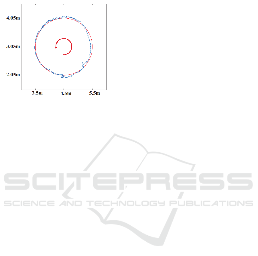
Figure 7: Real tracking results of the proposed algorithm.
Red: ideal path, blue: estimated path.
distortions. Despite of this error, the method was able
to track the object along the circle. The maximum
tracking error during the experiment was 0.14m,
while the average absolute error was 0.04m. The
method of (Zachár and Simon, 2014b) lost track
shortly after starting the circle (not shown in
Figure 7).
The computation complexity of the proposed
method is low: the calculation of the error map can be
restricted to the neighborhood of the estimated
previous position, thus the required time for the
position estimation is constant in each round and
independent of the measurement area. In the current
implementation the evaluation of a measurement set
takes less than 8ms in a 800x800 grid. Note that the
required operations can be highly parallelized.
The proposed method highly outperforms RSSI-
based methods, where the accuracy is in the range of
meters (Au et al., 2013), and its accuracy is
comparable to the best reported results of time of
flight radio systems (Ye et al., 2011).
5 CONCLUSIONS
In this paper a novel object tracking method was
proposed, which utilizes radio-interferometric phase
measurements. The proposed solution enhances the
robustness of the estimator and thus increases the
accuracy of the position estimations when multipath
effects, present in environment, cause distortions in
the phase map, and thus the real phase map is
different from the ideal one. The proposed method
utilizes an error surface, created from the unwrapped
ideal phase maps and the unwrapped measurement
values. The proposed method shows more robust
behavior when phase distortions are present. The
performance of the algorithm was illustrated by
simulations and real measurements.
The proposed error-surface based algorithm is a
significant step towards more robust radio-
interferometric tracking: the potential problem of
incorrect ideal phase map is correctly handled. The
proposed method, however, requires unwrapped
measured phase values, still presenting potential error
sources: when the unwrapping is inaccurate (e.g.
because of missing of faulty measurements) the
position estimate may permanently remain biased.
Future work includes self-correction mechanisms to
provide tolerance against faulty measurements as well.
REFERENCES
Au, A.W.S., et al, 2013. Indoor Tracking and Navigation
Using Received Signal Strength and Compressive
Sensing on a Mobile Device. IEEE Transactions on
Mobile Computing, Vol. 12, No. 10, pp. 2050–2062.
Dil B.J., Havinga, P.J.M., 2011. Stochastic Radio
Interferometric Positioning in the 2.4 GHz Range.
Proceedings of the 9th ACM Conference on Embedded
Networked Sensor Systems (SenSys 11), Seattle, WA,
pp. 108-120.
Lanzisera, S., Zats, D., Pister, K. S. J., 2011. Radio
Frequency Time-of-Flight Distance Measurement for
Low-Cost Wireless Sensor Localization. IEEE Sensors
Journal, Vol. 11, No. 3, pp.837-845.
Maroti M., et al, 2005. Radio Interferometric Geolocation.
In ACM Third International Conference on Embedded
Networked Sensor Systems (SenSys 05), San Diego,
CA, pp. 1-12.
Tribolet, J.M. , 1977. A new phase unwrapping algorithm.
IEEE Transactions on Acoustics, Speech, and Signal
Processing, Vol. 25, No.2, pp. 170-177.
Ye, T., Walsh, M., Haigh, P., Barton, J., O'Flynn, B., 2011.
Experimental impulse radio IEEE 802.15.4a UWB
based wireless sensor localization technology:
Characterization, reliability and ranging. 22nd IET Irish
Signals and Systems Conference ISSC 2011, Dublin,
Ireland, 23-24 Jun 2011.
Zachár, G., Simon, G., Maróti, M., 2014a. Radio
Interferometric Object Tracking. Proc. 8th
International Conference on Sensing Technology, ICST
2014, pp. 453-458.
Zachár, G., Simon, G., 2014b. Radio-Interferometric
Object Trajectory Estimation. Proc. 3rd International
Conference on Sensor Networks, SENSORNETS 2014,
pp. 268-273.
Zachár, G., Simon, G., 2015a. Radio Interferometric
Tracking Using Redundant Phase Measurements. Proc.
2015 IEEE International Instrumentation and
Measurement Technology Conference, I2MTC 2015,
pp.2003-2008.
Zachár, G., Simon, G., 2015b. Prediction-aided Radio-
SENSORNETS 2016 - 5th International Conference on Sensor Networks
212

interferometric Object Tracking. Proc. 4th
International Conference on Sensor Networks,
SENSORNETS 2015, pp. 161-168.
Towards Distortion-tolerant Radio-interferometric Object Tracking
213
