Power Management of Personal Computers based on User Behaviour

Brian Setz, Faris Nizamic, Alexander Lazovik and Marco Aiello

Distributed Systems Group, Johann Bernoulli Institute, University of Groningen,

Nijenborgh 9 (Bernoulliborg), 9747 AG, Groningen, The Netherlands

Keywords:

Context Aware Power Management, Timeout Optimization, Green Computing, Energy Efﬁciency.

Abstract:

It has been shown that up to 64 percent of personal computers in ofﬁce buildings are left running during after-

hours. Enabling power management options such as sleep mode is a straightforward method to reduce the

energy consumption of computers. However, choosing the right timeout can be challenging. A sleep timeout

which is too low leads to discomfort, whereas a timeout which is too high results in poor energy saving

efﬁciency. Having the users choose their own sleep timeout is not viable as research shows that most users

disable the sleep timeout completely, or choose a suboptimal timeout. Unlike existing context based power

management systems which use predeﬁned rules, we propose a solution which can determine a personalized

sleep timeout for any point in time solely based on the users behaviour. We propose multiple models which

have the goal of maximizing the energy savings while minimizing discomfort. The models are tested on the

computers of employees of the University of Groningen over several weeks. We analyse the results of the

experiments and determine which model performs best. We can potentially save between 4.02 and 17.17 kWh

per computer per year, depending on the model that used.

1 INTRODUCTION

A report from the Intergovernmental Panel on Climate

Change indicates that the increase in CO

levels in the

atmosphere is caused by human intervention with a

probability of over 90 percent (Solomon et al., 2007).

Their report shows that countries shall have to reduce

emission levels by 60 to 90 percent by 2050. If

not, temperatures will rise globally with more than 2

degrees Celsius by the end of 2050.

The IT sector is a large consumer of electricity

around the world according to a report by the climate

group on behalf of the Global eSustainability Initia-

tive. They state that between 2 percent and 10 percent

of the world wide energy consumption is attributed

to the IT sector (GeSI, 2008). Personal computers in

particular account for a large amount of the energy

consumption within modern buildings such as ofﬁces,

universities and libraries (Roth et al., 2002). In most

cases there is very little incentive to save energy for

the occupants of these types of buildings, since they

are not paying the electricity bills. Therefore, energy

savings without interfering with the user’s workﬂow

would be preferable.

It is common to encounter personal computers

which are powered on while they are not in use (idle).

While each individual computer does not consume

much energy, all idle computers combined do waste

a signiﬁcant amount of energy. Saving that energy by

putting idle computers to sleep appears to be an ob-

vious solution for decreasing energy consumption, as

sleep mode reduces the consumption by more than 95

percent. However, in practice it appears that putting

computers to sleep is not as common as one might

think, as in some cases up to 64 percent of personal

computers are still turned on after work-hours (Web-

ber et al., 2006).

In our research we aim to decrease the energy con-

sumption of personal computers by using the sleep

mode of these computers in an intelligent manner. We

believe this can be done more intelligently than ex-

isting solutions, as we can exploit the fact that users

leave their computers at certain times, for example

during lunch, or for meetings that take place regu-

larly. By learning these patterns we can predict that

their computer will be idle at certain time. Thus we

can adjust their personalized sleep timeout such that

their computers will go to sleep when they are away,

ultimately saving energy without causing discomfort.

The process to determine a personalized sleep

timeout is supported by the data which Sleepy col-

lects from computers. Sleepy is the context aware

power management software application which was

developed as a part of this research. The collected

Setz, B., Nizamic, F., Lazovik, A. and Aiello, M.

Power Management of Personal Computers based on User Behaviour.

In Proceedings of the 5th International Conference on Smart Cities and Green ICT Systems (SMARTGREENS 2016), pages 409-416

ISBN: 978-989-758-184-7

409

data is used as part of a learning process to ﬁnd the

optimal sleep timeout for individual users. The prob-

lem of ﬁnding the personalized sleep timeout can be

generalized as an optimization problem for sensors

which have some type of timeout that is inﬂuenced

by user behaviour. An optimal timeout is a time-

out that balances the beneﬁts and the costs that come

with a certain timeout setting. In this case, the time-

out is the sleep timeout of personal computers. The

costs and beneﬁts are user comfort versus energy sav-

ings. Three different models have been deﬁned in or-

der to ﬁnd the balance between the beneﬁts and costs

constraints. We use machine learning to learn linear

regression models using the linear least squares ap-

proach.

The approach we propose differs from existing so-

lutions as we dynamically build a proﬁle based on the

user’s behaviour and uses this to determine the opti-

mal sleep timeout at any given point in time. The ex-

isting context aware power management systems are

most commonly based on predeﬁned rules entered by

the user, or depend on speciﬁc hardware devices to

function optimally. We propose a solution which; 1)

does not require any manual actions from the user in

order to achieve energy savings, 2) can function on a

wide range of computers as it does not depend on spe-

ciﬁc hardware devices, and 3) aims to keep user com-

fort high and maintain the user’s productivity levels.

We perform experiments in order to verify the en-

ergy savings which could be achieved when using a

certain model. The experiments are performed on a

number of computers of the University of Groningen.

These computers are personal computers located in

the Bernoulliborg, which is home to the Faculty of

Mathematics and Natural Sciences.

The paper is organized as follows: Section 2

presents the background of this work and related

works. Section 3 describes the architecture of our so-

lution. Section 4 shows the results of using the solu-

tion in practice. Section 5 discusses the results and

future works.

2 BACKGROUND

In a study by (Webber et al., 2006) it is discovered

that up to 64 percent of all computers in ofﬁces are

still powered on during after-hours. Only 6 percent of

all computers made use of the available power man-

agement options, such as sleep mode. Of the moni-

tors attached to the computers around 75 percent were

powered on during after-hours. However, 66 percent

of all monitors used some form of power manage-

ment. We can conclude that there are signiﬁcant sav-

ings still to be made by putting computers to sleep. A

report from the Intergovernmental Panel on Climate

Change (Karayi, 2007) suggests that computers are

powered on and left unattended about 28 percent of

the time. The authors also show that 49 percent of

users never or rarely turn off their computer. Fur-

thermore, ﬁndings in (Chiaraviglio and Mellia, 2010)

also conﬁrm that computers are usually left powered

on. Their ﬁndings show that laptops are often turned

off, but the more power hungry desktop computers are

not. Up to 50 percent of these desktop computers are

still running during off peak hours. Of these comput-

ers, over 75 percent could be turned off in order to

achieve energy savings. According to (Nordman and

Christensen, 2009) the energy consumption of desk-

top computers is around 80 watts when idling. When

also including a 17-inch display monitor the energy

consumption increases to around 115 watts. Many

users already assume their computer has sleep mode

enabled, although in reality it is likely that the sleep

mode has in fact been disabled, as is indeed the case

at the University of Groningen.

These numbers show that there is a lot of potential

for energy savings in this area. Especially if these

savings could be achieved in an unobtrusive manner.

An issue that arises when putting computers to

sleep is that they are no longer available over the net-

work. This is an issue when users want to be able

to access their ﬁles remotely, and when IT adminis-

trators want to be able to manage computers at any

given time. In (Christensen and Gulledge, 1998) a

solution to this problem is proposed by introducing

Sleep Proxies. These proxies allow computers to have

a network presence while they are asleep. An actual

implementation of this concept is described in (Reich

et al., 2010). More research and information on the

topic of sleep proxies can be found in (Nordman and

Christensen, 2007), (Khan et al., 2012) and (Cheshire,

2008).

Windows Power Management Events are used by

the sleep proxy to detect changes in the power state of

the computer. We adopt this basic technique and use

this in our learning process. Sleep proxies themselves

do not adapt to the user’s behaviour. This is an aspect

which the solution presented in this paper attempts to

improve on.

Dynamic sleep timeout optimization is needed in

order to minimize the user impact of computers en-

tering sleep mode. In (Durand et al., 2013b) the

sleep time-outs of printers are dynamically changed

based on the time between print requests. The ap-

proach chosen in this research is to apply Hidden

Markov Models to create a statistical framework for

timeout optimization. More details regarding how

SMARTGREENS 2016 - 5th International Conference on Smart Cities and Green ICT Systems

410

to model power management using Markov Models

can be found in (Durand et al., 2013a) and in (Benini

et al., 1999).

There are software based solutions which also fo-

cus on Context Aware Power Management. One of

these software solution is PoliSave (Chiaraviglio and

Mellia, 2010). PoliSave works by allowing the user to

enter a schedule for their computer: the user can spec-

ify at which time and day the computer should per-

form some power management action such as sleep,

turn on or turn off. This allows for a great deal of

personalization of the power management on user-

basis. The authors indicate that usually 56 percent

of the computers they monitored were turned on at all

time. After applying their techniques this percentage

was reduced to 6 percent. The average daily uptime

of computers was reduced by more than 6 hours per

working day, from 15.9 hours to 9.7 hours. As a re-

sult savings of over 219 kWh per year were achieved

in their speciﬁc environment. The downside of the

approach taken by PoliSave is that the users need to

manually manage their schedule for the computers.

A different approach is taken by E-Net-Manager

(Brienza et al., 2014). The similarity between E-

Net-Manager and PoliSave is the fact that they both

use a schedule based approach to power management

in which the end user manually needs to enter the

schedule. The difference is that E-Net-Manager em-

ploys other sensors which determine whether a user

is present or not. These sensors include BlueTooth

sensors which take advantage of how the BlueTooth

handshake mechanism works. They also take advan-

tage of other wireless techniques such as using the

radio connectivity of smart-phones to determine the

presence of speciﬁc users. The computer is turned on

and off based on this presence. The manual calender

based schedule is there for back-up in this case. An-

other software based solution for power management

is Gicomp (Jarus and Oleksiak, 2013). Gicomp real-

izes a centralized power management platform. The

software is able to change the power management pol-

icy of large numbers of personal computers simulta-

neously. The software, however, does not allow per-

sonalization of power management policies.

Our solution does not attempt to take over control

of the operating system, instead it lets the operating

system decide whether the computer is in use or if it is

not. We also reuse the built in sleep timeout system of

the operating system and optimize it by personalized

timeout adjustments. The advantage of this approach

is that computers are only put into sleep mode when

they are not actually used. Furthermore, our approach

does not require predeﬁned rules and schedules, in-

stead it adapts to the user in an automatic, unobtrusive

manner. And ﬁnally, the system we propose does not

have any speciﬁc hardware requirements; it works on

every personal computer.

3 ARCHITECTURE

As part of this research a software application is de-

veloped, named Sleepy. This application manages the

sleep timeout of personal computers and monitors the

computer usage. The sleep timeout determines when

the computer enters sleep mode after being idle for

a set amount of time. Sleepy also monitors and col-

lects data from the computers on which it is installed.

Before we take a closer look at the models, we have

to understand the data sets on which the models are

based.

3.1 Data Set

The data set used in our research is obtained by mon-

itoring computers for an extended period of time us-

ing the Sleepy-software. For each computer three dif-

ferent types of data are collected: state data, activity

data, feedback data. The way Sleepy collects this in-

formation about the state of a computer is by listening

to System Power Management events.

State Data - State data gives insight into the state

of the computer. The state refers to the power man-

agement state of the computer and can assume three

values: On, Sleeping and Off.

Activity Data - Activity data is collected in order

to detect if a computer is actually being used while it

is turned on. The activity value can be either Active,

Idle or Inactive. Active means the computers is ac-

tively being used, whereas idle means the computer is

turned on but not in use. A computer is inactive when

it is turned off. Sleepy monitors the activity of the

computer by reading the LASTINPUTINFO structure.

Feedback Data - Feedback is collected in order to

determine whether Sleepy is working with a minimal

user impact. We only collect negative feedback, and

we react immediately as soon as negative feedback is

received. As a result the user does not have to provide

any feedback when everything is working as expected

but only when things are not working as they should.

Users can explicitly report their feedback using a tray

icon presented by Sleepy in the system tray. Right

clicking on this tray icon provides the user with the

menu option to disable Sleepy until reboot. When this

menu option is selected the user will be shown a dia-

Sleepy. When a computer enters sleep mode and is

woken up before a certain time has passed it is also

Power Management of Personal Computers based on User Behaviour

411

considered negative feedback as this could mean that

the sleep timeout was too low. The information about

the length of a sleep period can be extracted from the

state data set.

Activity Probability - The activity probability is

based on the activity data set. It represents the proba-

bility that a certain computer is actively being used at

a given moment in time. This probability is calculated

by looking at the historical activity data of the same

day of the week, over the past few weeks.

Idle Time - Idle time can also be extracted from

the activity data set. It is trivial to determine the idle

time of a computer: the current state of the computer

can be determined by looking at the most recent value

in the activity data set. If this activity state is idle then

the idle time is simply the amount of time since the

activity state changed to idle. Using the idle time one

can determine how long it has been since the com-

puter has been actively used.

3.2 Models

Three models have been deﬁned to optimize the sleep

timeout. These models share a common goal: to min-

imize the amount of time in which a computer is in

the idle state. Reducing this idle period is done by

putting the computer to sleep. In turn, putting com-

puters to sleep leads to energy savings. However, it is

important that the negative feedback remains minimal

to maintain a high level of user comfort and produc-

tivity.

In order to determine the performance of each

model they are graded according to some cost func-

tion. The cost for choosing a certain sleep timeout

can only be determined after a certain amount of time

has passed, as negative feedback is not always instan-

taneous. The cost function for determining the per-

formance of the model for a given timespan is deﬁned

as:

idle

= {z ∈ A

|z = idle} (1)

E(t) =

∑

z∈A

idle

z + (1 +

N(t)

h(t)

)N(t) (2)

∑

z∈A

idle

z + N(t) +

N(t)

h(t)

(3)

Where A

is the set of activity data containing

time intervals for every activity change for timespan t.

idle

is the set of activity data only containing the time

intervals during which the activity was idle. N(t) rep-

resents the negative feedback collected for timespan

’t’. h(t) is the hours of sleep measured for the given

timespan. It can be argued that an increase in negative

feedback (decrease in user comfort) is more costly

than an increase in idle time (decrease in energy sav-

ings), therefore

N(t)

h(t)

, the ratio of negative feedback

per hours of sleep, is used to adjust this cost. This

ratio an indication of how expensive in terms of dis-

comfort each hour of sleep is. E(t) is the resulting

cost for the given model over timespan ’t’.

Three concrete models have been developed based

on three different types of data: activity probability,

negative feedback and idle time. The models return

a personalized sleep timeout for a given time, s(t),

returning the sleep timeout in minutes, where t is an

instant in time. The ﬁrst model is a rule based model

whereas the remaining two models are linear regres-

sion models. The weights for these linear regressions

models (denoted as w

) are obtained using linear re-

gression.

The goal of Model 1 is to have a high sleep time-

out whenever there is a chance of user activity at that

given moment in time. The sleep timeout becomes

low when there is a low probability of user activity.

s(t) =

(

max

, if P

(t) > ε.

min

, otherwise.

(4)

• P

(t) – Activity probability at time t

• ε – Activity threshold

• s

min

– Minimum sleep timeout value

• s

max

– Maximum sleep timeout value

The goal of Model 2 is to ﬁnd the most optimal

sleep timeout based on two different input parame-

ters: activity probability and negative feedback.

s(t) = w

(t) + w

N(t) + w

(5)

• P

(t) – Activity probability at time t

• N(t) – Negative feedback count at time t

A higher activity probability should lead to an in-

crease of the sleep timeout, if the probability of a

computer being in use is high it should not enter sleep

mode. Furthermore, an increase in negative feedback

should also lead to an increase of the sleep timeout.

The difference is that an increase in negative feed-

back should increase the sleep timeout more than an

increase in activity probability. The negative feedback

at time t also includes negative feedback received be-

fore time t.

The goal of Model 3 is to ﬁnd the most optimal

sleep timeout based on three different input parame-

ters: activity probability, negative feedback and idle

time.

s(t) = w

(t) + w

N(t) + w

I(t) + w

(6)

SMARTGREENS 2016 - 5th International Conference on Smart Cities and Green ICT Systems

412

• P

(t) – Activity probability at time t

• N(t) – Negative feedback count at time t

• I(t) – Idle time in minutes at time t

The ﬁrst two parameters of this model work ac-

cording to the same principles as described for Model

2. The third parameter, idle time, also increases the

sleep timeout as its own value increases. The rate of

increase should be somewhere in between those of the

ﬁrst two parameters.

4 EXPERIMENTS

Experiments have been performed to determine the

effectiveness of the three different models previously

deﬁned. The experiments were performed over the

course of three weeks, starting on the 1st of June 2015

and ending on the 22nd of June 2015. These dates

were chosen such that no holidays occurred during

the experiments, to prevent skewed results. Our so-

lution was deployed two months prior, in April 2015,

in order to begin the collection of data and test the

stability in the operating environment.

A total of fourteen computers were part of the ex-

periments. These are computers used by staff mem-

bers in the Bernoulliborg, a building of the University

of Groningen. These staff members include; profes-

sors, lecturers and researchers but also faculty staff.

By including staff members with different roles we

try to simulate a realistic environment and test if our

solution is still effective when the user’s activity is

less predictable. The participants were split into three

groups. For each week, each group tested a different

model. Each model has been tested and evaluated for

exactly six days, starting on Monday and ending on

Saturday. The seventh day of the week, Sunday, was

used for transitioning between models.

4.1 Computer Usage Proﬁling

Predicting when a computer will be in use is a very

important aspect when determining the personalized

sleep timeout. Each of the three models take this into

account by calculating the activity probability. The

activity probability represents the probability of see-

ing activity on a computer at a certain moment in

time. A usage proﬁle can be generated by calculat-

ing the activity probability at multiple points during a

given time interval.

The data appears to have a weekly seasonality as

users often work on the same days every week. There-

fore, historical data from the same day of the week

is used to predict the future activity. Data from up to

four weeks ago is used in the prediction of the activity

probability. When predicting the activity probability

for a certain moment in time a window of ten min-

utes is used. Equation 7 shows how the proﬁles are

calculated.

activity

(t) =

∑

i=1

f (t − weeks(n))

f (t) =

(

0, if no activity

1, if some activity

(7)

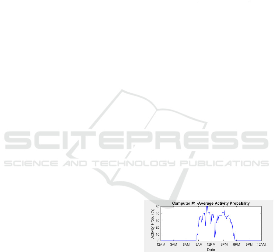
The proﬁles shown in the following ﬁgures are the

average proﬁle of all three weeks. The probability

ranges anywhere from zero to one hundred percent.

Where zero percent indicates there is no predicted ac-

tivity, and one hundred percent indicating that there is

a probability of a hundred percent of seeing activity.

These average proﬁles were generated by combining

the daily proﬁles. A number of patterns can be seen

in most of the proﬁles, where the activity probability

drops at certain times. The most common drop oc-

curs at around 1 PM. This can be explained by users

leaving their computer for their lunch break. Another

common pattern is a drop in the activity probability

around 10 PM or 11 PM. Another pattern that can also

be seen in the activity proﬁles is that most users use

their computer almost exclusively between 8AM and

7PM. Both these patterns can be seen in Figure 1, Fig-

ure 2 and Figure 3. The patterns verify that there are

indeed opportunities to save energy, even if users shut

down their computer at the end of every day. Assum-

ing an average working day of eight hours and a lunch

break of thirty minutes means that the computer could

potentially sleep for at least 6.25% of the time during

a full working day.

Figure 1: Computer 1 - average activity probability.

4.2 Results

For the experiments the following parameters have

been set for Model 1: the minimum sleep timeout s

min

is ﬁve minutes. The maximum sleep timeout s

max

sixty minutes. The activity threshold ε is set to a value

of 0.05, or 5 percent.

For determining the initial timeout we use train-

ing data that is based on expert knowledge of which

Power Management of Personal Computers based on User Behaviour

413

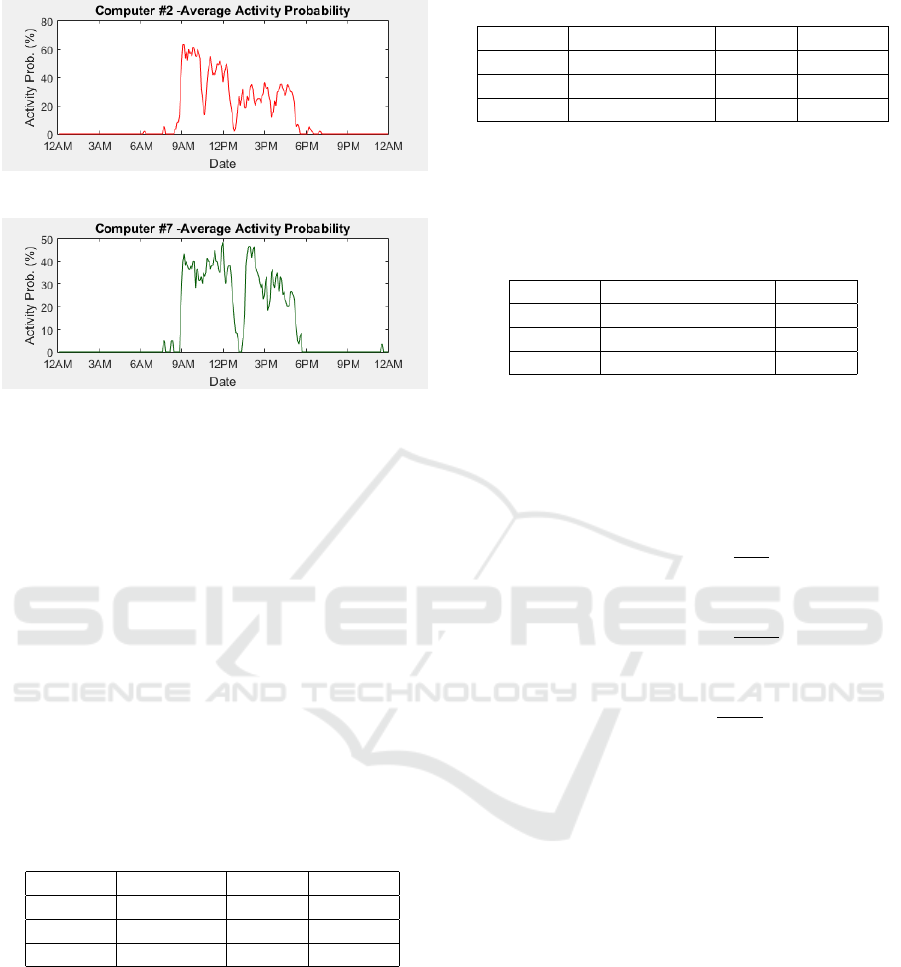
Figure 2: Computer 2 - average activity probability.

Figure 3: Computer 7 - average activity probability.

timeout should be associated to the given input pa-

rameters. It allows us to have a reasonable sleep time-

out to start with, and prevent negative feedback that

would be associated with a complete cold start. The

data is split into training data and test data. Sixty per-

cent of the data is used for training and the remain-

ing fourty percent is used to test the trained model.

Once this model has been trained it is automatically

adjusted based on the parameters. Spark MLlib pro-

vided the implementation for solving these regression

problems.

Table 1 shows the idle time per model in hours,

and also the average idle time per computer. Model

3 becomes more aggressive, with regards to decreas-

ing the sleep timeout, the longer a computer is idle.

Therefore it is as expected that this model has the least

amount of idle time.

Table 1: Total idle time in hours per model.

Model Hours Idle Per PC Std. dev.

Model 1 31.19h 2.60h 1.73

Model 2 27.05h 2.25h 1.76

Model 3 19.57h 1.63h 1.56

The exact number of hours of sleep for each model

are shown in Table 2. Using Model 2 or Model 3 re-

sults in over four times as many hours of sleep com-

pared to Model 1. The difference in hours of sleep is

due to the fact that the ﬁrst model puts the computer to

sleep when there is almost zero probability of seeing

activity. Which means that there are fewer moments

when it puts the computer to sleep, when compared

to the other two models. The second and third models

are more aggressive when with regards to determining

the sleep timeout, and therefore result in more hours

of sleep.

Table 2: Total sleep in hours per model.

Model Hours Sleeping Per PC Std. dev.

Model 1 5.54h 0.46h 0.42

Model 2 22.26h 1.85h 2.29

Model 3 23.68h 1.97h 3.17

An overview of the negative feedback occurrences

can be seen in Table 3. Model 1 did not generate any

negative feedback. This can be explained by the fact

that this model is the least aggressive model.

Table 3: Negative feedback occurances.

Model Negative Feedback Per PC

Model 1 0 0.0

Model 2 11 0.917

Model 3 14 1.167

We can apply the previously deﬁned cost func-

tion (eq. 3) to determine the ranking of each model.

A lower score means that the model performs better.

We can input the values for the idle time, the negative

feedback and hours of sleep. The equations for each

model become:

model1

(t) = 31.19 + 0 +

5.54

= 31.19 (8)

model2

(t) = 27.05 + 11 +

22.26

= 43.48 (9)

model3

(t) = 19.57 + 14 +

23.68

= 41.84 (10)

These results show that model 1 is the optimal

model in terms of minimizing user discomfort.

The energy consumption of a computer is around

115 watts according to Nordman et al (Nordman and

Christensen, 2009). According to Roberson et al

(Roberson et al., 2002) the power consumption of

desktop computers is around 105 watts. In (Bluejay,

2012) the authors conclude that the energy consump-

tion of computers ranges anywhere from 77 watts to

322 watts. All sources agree that the power consump-

tion when sleeping is around 5 watts. In the follow-

ing calculations we shall use 150 watts as the average

power consumption. This is based on measurements

taken from computers in the Bernoulliborg. Further-

more, we shall use the energy tariffs in the Nether-

lands, which is 22 eurocents per kilowatt-hour (Mileu

Centraal, 2015a) at the time of writing.

The number of computers in the Bernoulliborg is

estimated to be around 500. This estimation is based

on the fact that there is room for 350 employees,

where we assume at least one computer per employee.

We also have to include the number of computers for

SMARTGREENS 2016 - 5th International Conference on Smart Cities and Green ICT Systems

414

students, this number is estimated to be around 150.

This is based on the fact that there are six large com-

puter rooms on the second ﬂoor with around 25 com-

puters each.

The amount of sleep per computer per month is

shown in Table 4. The difference between Model 1

and the other models is signiﬁcant: Model 1 results in

only 2.31 hours of sleep whereas both other models

result in 9 to 10 hours of sleep. The monthly hours

of sleep were calculated by multiplying the sleep per

computer times 5. This is because the hours of sleep

per computer was taken over a 6 day period. It is im-

portant to know the number of hours a computer is

asleep in order to determine the monthly kWh savings

per model.

Table 4: Sleep per month in hours.

Model Total Sleep Per PC PC per Month

Model 1 5.55h 0.46h 2.31h

Model 2 22.26h 1.85h 9.27h

Model 3 23.68h 1.97h 9.87h

To determine the monthly energy savings we have

to determine two things: the kWh consumed per com-

puter while it was sleeping and the kWh the computer

would have consumed if it would have been turned on

instead of asleep. These numbers can be seen in Table

Table 5: kWh consumption per month per computer.

Model Sleeping Turned On Savings

Model 1 0.012 kWh 0.35 kWh 0.33 kWh

Model 2 0.046 kWh 1.39 kWh 1.35 kWh

Model 3 0.049 kWh 1.48 kWh 1.43 kWh

Over the course of a year the savings per computer

add up to a signiﬁcant number as can be seen in Ta-

ble 6. Even using Model 1 saves around 4 kWh per

computer per year. This equals to around 90 euro-

cents worth of energy savings per computer per year.

Using Model 2 or Model 3 results in 16 to 17 kWh of

energy savings, or 3.55 euro to 3.77 euro of economic

savings.

Table 6: Estimated annual savings per computer.

Model Savings per PC Savings per PC

Model 1 4.02 kWh e0.89

Model 2 16.13 kWh e3.55

Model 3 17.17 kWh e3.77

Finally, let us take a look at the annual savings that

could be achieved in an actual ofﬁce building. The

results for the Bernoulliborg can be seen in Table 7.

If all computers in Bernoulliborg used Model 1 then

the annual savings would be 2010.68 kWh, which

amounts to 442.35 euro. The biggest savings can be

achieved using Model 3: the savings are 8583.49 kWh

or 1888.37 euro.

Table 7: Estimated annual savings in Bernoulliborg.

Model Savings (kWh) Savings (euro)

Model 1 2010.68 kWh e442.35

Model 2 8067.44 kWh e1774.84

Model 3 8583.49 kWh e1888.37

5 CONCLUSION AND FUTURE

WORK

We have looked at how context aware power man-

agement based on user behaviour can be implemented

and used in practice. We have also looked at several

different models and the savings which were achieved

by each of these models by performing experiments

over the course of a month. Considering the number

of typical ofﬁce buildings around the world, the num-

ber of computers used, and the potential savings per

computer, if this solution were widely applied its en-

vironmental impact would be signiﬁcant.

Besides measured savings, our solution provides

valuable additional information about computer usage

in a workspace. Using this information we can in-

troduce additional savings for other control solutions

by increasing the sensor data accuracy. For instance,

computer usage information provides higher accuracy

of algorithms for presence and activity recognition

that are used for lighting, appliances and heating con-

trol.

Furthermore the research opens an interesting area

to which other machine learning techniques can be

applied. Instead of using linear regressions models

one can also look at other methods of modelling a per-

sonalized sleep timeout. A good candidate would be

to explore the possibilities that reinforcement learn-

ing offers. We plan to improve on a number of points

in our future work. The experiments were performed

on fourteen computers of staff members in a building

of the University of Groningen.

For more statistically signiﬁcant results, we will

repeat the experiments on a larger sample of computer

which contain more different types of users. More-

over, it will be interesting to compare the results from

staff member computers with those from the publicly

available student computers. Besides energy and eco-

nomic savings, we will investigate the proposed solu-

tion from the perspective of user acceptability.

By deploying our solution on a number of com-

puters within the Bernoulliborg we were able to save

energy quite effectively, allowing us to save up to

17.17 kWh per year per computer. These savings

Power Management of Personal Computers based on User Behaviour

415

were achieved despite the fact that the environment

in which we performed the experiments was already

reasonably energy efﬁcient, as all participants turned

their computer off during off-peak hours. The amount

of energy saved within building Bernoulliborg, when

using Model 3 for a year on all computers, would be

8583.49 kWh. Which is enough energy to power an

average sized Dutch household for almost two and a

half years (Mileu Centraal, 2015b).

ACKNOWLEDGEMENTS

We thank Marco Wiering for his feedback, support,

and the valuable discussions regarding the models.

We also thank Tuan Anh Nguyen for numerous dis-

cussions and active involvement. Furthermore we

thank Ronald Zwaagstra for providing equipment for

our development process, as well as to the CIT per-

sonnel for their support with deploying our solution

in the Bernoulliborg building of the University of

Groningen. The work is supported by The Nether-

lands Organisation for Scientiﬁc Research NextGenS-

mart DC project, contract no. 629.002.102.

REFERENCES

Benini, L., Bogliolo, A., Paleologo, G., and Micheli, G. D.

(1999). Policy optimization for dynamic power man-

agement. 18:813–833.

Bluejay, M. (March 2012). How much electricity do com-

puters use? http://michaelbluejay.com/electricity/

computers.html.

Brienza, S., Bindi, F., and Anastasi, G. (2014). E-net-

manager: A power management system for networked

pcs based on soft sensors. In Smart Computing

(SMARTCOMP), 2014 International Conference on,

pages 104–111. IEEE.

Cheshire, S. (February 2008). Method and apparatus for

implementing a sleep proxy for services on a network.

United States Patent N. 7,330,986.

Chiaraviglio, L. and Mellia, M. (2010). Polisave: Efﬁ-

cient power management of campus pcs. In Software,

Telecommunications and Computer Networks (Soft-

COM), 2010 Int. Conference on, pages 82–87.

Christensen, K. J. and Gulledge, F. B. (1998). En-

abling power management for network-attached com-

puters. International Journal of Network Manage-

ment, 8(2):120–130.

Durand, J.-B., Girard, S., Ciriza, V., and Donini, L. (2013a).

Optimization of power consumption and device avail-

ability based on point process modelling of the request

sequence. Journal of the Royal Statistical Society: Se-

ries C (Applied Statistics), 62(2):151–165.

Durand, J.-B., Girard, S., Ciriza, V., and Donini, L. (2013b).

Optimization of power consumption and user impact

based on point process modeling of the request se-

quence. Journal of the Royal Statistical Society Series

C, 62(2):151–165.

GeSI (2008). Smart2020: Enabling the low carbon econ-

omy in the information age. The Climate Group -

Global eSustainability Initiative.

Jarus, M. and Oleksiak, A. (2013). Gicomp and greenof-

ﬁce monitoring and management platforms for it and

home appliances. In Pierson, J.-M., Da Costa, G.,

and Dittmann, L., editors, Energy Efﬁciency in Large

Scale Distributed Systems, volume 8046 of Lecture

Notes in Computer Science, pages 58–62. Springer

Berlin Heidelberg.

Karayi, S. (2007). Pc energy report 2007. http://

www.1e.com/energycampaign/downloads/1E%20

Energy%20Report%20US.pdf.

Khan, R., Bolla, R., Repetto, M., Bruschi, R., and

Giribaldi, M. (2012). Smart proxying for reducing

network energy consumption. In Performance Eval-

uation of Computer and Telecommunication Systems

(SPECTS), 2012 Int. Symposium on, pages 1–8.

Mileu Centraal (2015b). Gemiddeld energieverbruik. http://

www.milieucentraal.nl/energie-besparen/snel-besparen/

grip-op-je-energierekening/gemiddeld-energieverbruik/.

Mileu Centraal (July 2015a). Energieprijzen. http://

www.milieucentraal.nl/energie-besparen/snel-besparen/

grip-op-je-energierekening/energieprijzen/.

Nordman, B. and Christensen, K. (July 2009). Greener pcs

for the enterprise. IEEE IT Professional.

Nordman, B. and Christensen, K. (October 2007). Improv-

ing the energy efﬁciency of ethernet-connected de-

vices: A proposal for proxying. Ethernet Alliance.

Reich, J., Goraczko, M., Kansal, A., and Padhye, J. (2010).

Sleepless in seattle no longer. In USENIX Annual

Technical Conference. USENIX.

Roberson, J. A., Homan, G. K., Mahajan, A., Nordman, B.,

Webber, C. A., Brown, R. E., McWhinney, M., and

Koomey, J. G. (July 2002). Energy use and power

levels in new monitors and personal computers. Envi-

ronmental Energy Technologies Division.

Roth, K., Goldstein, F., and Kleinman, J. (January 2002).

Energy consumption by ofﬁce and telecommunica-

tions equipment in commercial buildings volume i:

energy consumption baseline. National Technical In-

formation Service (NTIS), US Department of Com-

merce, Springﬁeld, VA, 22161.

Solomon, S., Qin, D., Manning, M., Chen, Z., Marquis,

M., Averyt, K., Tignor, M., and Miller, H. (October

2007). Climate change 2007: The physical science ba-

sis. Cambridge University Press, Cambridge, United

Kingdom and New York, NY, USA.

Webber, C. A., Roberson, J. A., McWhinney, M. C., Brown,

R. E., Pinckard, M. J., and Busch, J. F. (2006). After-

hours power status of ofﬁce equipment in the usa. En-

ergy, 31(14):2823 – 2838.

SMARTGREENS 2016 - 5th International Conference on Smart Cities and Green ICT Systems

416