A Novel Technique for Point-wise Surface Normal Estimation

Daniel Barath

1,2

and Ivan Eichhardt

1,2

MTA SZTAKI, Budapest, Hungary

otv

os Lor

and University, Budapest, Hungary

Keywords:

Surface Normal Estimation, Afﬁne Transformation, Stereo Reconstruction, Oriented Point Cloud, Planar

Patch.

Abstract:

Nowadays multi-view stereo reconstruction algorithms can achieve impressive results using many views of

the scene. Our primary objective is to robustly extract more information about the underlying surface from

fewer images. We present a method for point-wise surface normal and tangent plane estimation in stereo

case to reconstruct real-world scenes. The proposed algorithm works for general camera model, however, we

choose the pinhole-camera in order to demonstrate its efﬁciency. The presented method uses particle swarm

optimization under geometric and epipolar constraints in order to achieve suitable speed and quality. An

oriented point cloud is generated using a single point correspondence for each oriented 3D point and a cost

function based on photo-consistency. It can straightforwardly be extended to multi-view reconstruction. Our

method is validated in both synthesized and real tests. The proposed algorithm is compared to one of the

state-of-the-art patch-based multi-view reconstruction algorithms.

1 INTRODUCTION

Estimation of surface normal and the related planar

patch has been an intensively researched area of com-

puter vision since decades. The aim of this paper is

to deﬁne a method and describe the theory behind, to

estimate planar-like spatial patches (surﬂets) for each

point correspondence in stereo case. We will show

that the proposed method can achieve more accurate

results in many cases than standard estimation tech-

niques, and it will be a powerful basis for subsequent

dense reconstruction algorithms. In our experience,

most of the sparse or dense reconstruction methods

estimate the spatial positions of the observed points

accurately, but they give rough estimations for the

patch orientations (the surface normals) most of the

time. This motivated our current work.

The algorithm assumes that 2D correspondences

(2D point pairs) are already established between im-

ages of a stereo pair. The calibration of the cameras

in the stereo setup should also be known. We assume

that the observed corresponding point pair belongs to

the same surﬂet. After triangulating the position of

this observed point from the known 2D point corre-

spondences, our algorithm further provides informa-

tion about the underlying surface: the tangent plane at

the point. The output of our algorithm is an oriented

point cloud, a sparse reconstruction of the scene.

1.1 Related Work

Stereo matching and reconstruction methods can be

classiﬁed into four different classes, based on their

applied model for the surface: voxel-based (Faugeras

and Keriven, 2002; Pons et al., 2007), deformable

polygonal (Zaharescu et al., 2007), depth-map fusion

(Strecha et al., 2006) and patch-based (Furukawa and

Ponce, 2010; Habbecke and Kobbelt, 2007) methods.

Since ours is patch-based, in the rest of the related

work we restrict ourselves to this class of methods.

Each patch is built from a local area and the tan-

gent plane of the surface. The tangent plane estima-

tion can be performed directly or indirectly. Direct

parametrization of a cost function with the parameters

of the tangent plane is an algebraic problem, where

the solution is the minimum of the cost function. Indi-

rectly, when a relative (afﬁne) homography is ﬁrst es-

timated between the projections of the 3D surﬂet, the

parameters of the tangent plane (and the surface nor-

mal) are expressed from this relation (Faugeras and

Lustman, 1988). Applied number of views and the na-

ture of the reconstruction (dense or sparse) may vary

among the direct or indirect methods.

Such an indirect approach is the work of

(Megyesi et al., 2006). Their method requires rec-

tiﬁed images to compute the scene structure in two

steps. It ﬁrst generates seed points using afﬁne patch-

688

Barath, D. and Eichhardt, I.

A Novel Technique for Point-wise Surface Normal Estimation.

DOI: 10.5220/0005776406860693

In Proceedings of the 11th Joint Conference on Computer Vision, Imaging and Computer Graphics Theory and Applications (VISIGRAPP 2016) - Volume 3: VISAPP, pages 688-695

ISBN: 978-989-758-175-5

matching, then propagates the estimated surface un-

der a set of conditions. On the seed points they use

exhaustive search (ES) to ﬁnd an optimal 3-DoF afﬁne

transformation between patches of the rectiﬁed views

based on a photo-consistency measure ﬁrst, then the

decomposition of these transformations results in sur-

face normals and disparity. The authors introduce

several epipolar geometry-based constraints in order

to narrow the search-space. Their normal visibility

constraint declares that normals pointing away from

the image planes or close to perpendicular to the prin-

cipal axis can be discarded.

There are several image-based surface nor-

mal estimation methods available, such as afﬁne

transformation-based technique (Barath et al., 2015)

or decomposition of the homography (Faugeras

and Lustman, 1988). The study of (Moln

ar and

Chetverikov, 2014) also showed that the surface nor-

mal can be expressed directly from the afﬁne homog-

raphy using the spatial gradients of the 2D projective

functions in the stereo setup. These approaches re-

quire full camera calibration and the (afﬁne) homog-

raphy related to the observed point pair.

Some other methods (Habbecke and Kobbelt,

2006; Furukawa and Ponce, 2010; Lhuillier and

Quan, 2005; Vu et al., 2012) can be classiﬁed as di-

rect methods for tangent plane estimation. In the

work of (Habbecke and Kobbelt, 2006), the authors

pose the problem as a plane search in 3D space. This

is similar to our approach, but unlike us, they work

with matched 2D blobs, and the proposed solution

optimizes the plane through 3 parameters. Gauss-

Newton optimization with a photo-consistency-based

cost function is used to solve the problem.

From the ﬁeld of multi-view dense reconstruction

we have to mention PMVS (Furukawa and Ponce,

2010). Their method is a patch-based 3-step – match,

expand and ﬁlter – procedure generating an oriented

point cloud (or patches), where the last two steps are

repeated n times. Matching is based on minimizing

a photometric discrepancy function, therefore, they

also optimize in both spatial and image space. Af-

ter initial matching, for patch optimization they use a

gradient method to reﬁne the orientation. In the ﬁl-

tering step the authors use a weak form of regular-

ization, where they apply visibility-based constraints

to eliminate incorrect matches and outliers. These

constraints show similarities to (Megyesi et al., 2006)

and to our approach, but in our method similar con-

straints are directly applied to the search space, not

as a post-processing step. The expansion step can be

related to the surface propagation step of (Megyesi

et al., 2006). As a ﬁnal step, of PMVS they also

generate a polygonal mesh through Poisson Surface

Reconstruction (Kazhdan et al., 2006) and an Itera-

tive Snapping step. In the latter, they enforce fore-

ground/background segmentation through energy op-

timization. The weakness of this method comes from

initialization of the surface normal (which prefers

fronto-parallel patches). As the patch orientation

moves away from fronto-parallel, the result of the gra-

dient method gets worse.

There are also a number of multi-step pipelines

working on massive number of views (Lhuillier and

Quan, 2005; Vu et al., 2012) to achieve high-quality

reconstruction. Their ﬁrst step is usually a crucial

one: building an initial sparse or quasi-dense recon-

struction of the scene (e.g. oriented point cloud).

Particle Swarm Optimization (PSO) (Kennedy,

2010; Shi and Eberhart, 1998) is a population-based

algorithm, designed to ﬁnd useful solutions for con-

tinuous problems in a bounded (or periodic) search

space. It is an iterative algorithm trying to ﬁnd and

improve candidate solutions. Multiple particles coop-

erate seeking one or multiple optima simultaneously.

PSO is derivative-free and copes well with noise.

1.2 Motivation and Goals

Establishing correspondences between stereo (or

multi-view) images is an ambiguous, the reconstruc-

tion of the underlying surface an ill-posed problem.

There are a number of methods applying constraints

and using several views to restrict the problem.

In this paper, we use a direct approach and formu-

late afﬁne patch-matching in such a way that the 2-

DoF search space is the same as the parameter space

of the surface normal of the corresponding surﬂet.

We preferred using PSO since unlike Gauss-Newton

methods, it attempts ﬁnding a global optimum with-

out derivatives. However, PSO has – in general – no

proof of convergence, in our formulation the quality

of the estimated tangent plane is at least as good as

if we used a coarse regular grid-based ES. Using the

epipolar geometry and direct constraints on the search

space, our algorithm opens up a novel way to address

high quality reconstruction from photos taken from

uncalibrated viewpoints.

This paper and also the algorithm do not deal with

full reconstruction. It focuses on individual tangent

plane estimation in order to provide a basis for a fu-

ture multi-view reconstruction algorithm. Potential

applications are in the ﬁeld of 3D reconstruction: gen-

erating seed points for surface-propagation, enhanc-

ing motion-from-structure in a multi-view setup.

Even though, the commonly used warp function is

homography for similar tasks, we chose afﬁne trans-

formation. The beneﬁt of building an afﬁne transfor-

A Novel Technique for Point-wise Surface Normal Estimation

689

mation from projection function gradients is, that it

is valid for any camera model. We already discussed

the simple pinhole-camera based formulation, but e.g.

extending the pinhole camera model and its projection

function with radial and tangential distortion gives the

following advantages.

1. No undistortion of input photos is needed.

2. When warping image patches, no evaluation of

camera distortion is needed for each pixel. The

afﬁne warp matrix is pre-evaluated, thus trans-

forming the patch is a fast afﬁne image warp.

3. The extension to (not discussed here) omnidirec-

tional cameras is also simple.

Although our afﬁne matching-based algorithm resem-

bles the seed point generation step of different method

(Megyesi et al., 2006) with ES, due to our novel for-

mulation of the matching problem, we are able to

substitute ES with a search heuristic (PSO), and no

rectiﬁcation of the input images is needed. Remark

that the estimation of the afﬁne transformation in their

work has 3-DoF since the images are rectiﬁed before-

hand. To our knowledge, applying PSO to reconstruc-

tion problems (Cagnoni, 2008) such as the topic of

this paper is new. Also, novel visibility constraints

dramatically restrict the search space of PSO.

We performed experiments on synthetic and real

data and compared our results to a state-of-the-art

method (Furukawa and Ponce, 2010) applied on a

stereo image pair as it can be seen in Sec. 4.1.1.

Poisson surface reconstruction (Kazhdan et al., 2006)

of the output of our method gives satisfactory qual-

ity without any post-processing or surface propaga-

tion (Megyesi et al., 2006) techniques.

The rest of this study is organized as follows: the

Sec. 2 describes the notations used in this paper and

the geometric background. Then, in Sec. 3 the core

of the proposed algorithm is written in the form of its

geometric representation and with novel constraints

on the search space, as well. Finally, in Sec. 4 we

show that our algorithm works well in synthetic and

real tests, and we conclude our research in Sec. 5.

2 NOTATIONS AND GEOMETRIC

BACKGROUND

In this work matrices are denoted by bold capitals

such as K or R, and vectors are underlined such as

, p, q, x. In addition, the notation P usually means a

point in 3D, p is usually a 2D projection on an image

plane and its homogeneous equivalent is ˜p.

The projection matrix of the perspective camera

model is denoted as P = K ·



R | T



∈ R

3×4

, and

Figure 1: Surface point with normal vector and tangent

plane.

constructed using the matrix of intrinsic camera pa-

rameters K ∈ R

3×3

, rotation matrix R ∈ R

3×3

and

translation vector T .

Conversion of a direction x ∈ R

to Spher-

ical coordinates is expressed as Sph (x) =

arccos





arctan

(Y, X)

Let a, b ∈ R

, such that ∀i ∈

{

1, 2

}

: a

≤ b

then rect [a, b] is the minimum (axis-aligned) rectan-

gle containing vectors a and b.

3 ITERATIVE TANGENT PLANE

ESTIMATION

In this section we show that the normal vector

can be robustly estimated from only a single point-

correspondence, and its local environments on the

ﬁrst, and the second images. Let us denote the pro-

posed method with ITPE in the latter sections.

3.1 Basis of the Algorithm

The main idea behind the proposed algorithm is very

simple: if a point of a surface is given, the tangent

plane of the observed point can be described by the

normal vector of the plane as it can be seen in Fig. 1.

It means exactly that the DoF of this plane is two since

it can be parametrized by spherical coordinates (u, v)

(omitting the third, radial coordinate). Let us denote

the stereo camera setup with the projection matrices

of the cameras P

, P

, and the i

3D point with

homogeneous form. Its projections on the two cam-

eras are p

, p

. Now the tangent plane of the ob-

served point can be deﬁned by the point and normal

n. The problem is reduced to a two-dimensional box-

constrained optimization, where the unknown param-

eters are u and v; therefore it always has a solution.

In order to choose the best candidate surface nor-

mal we use weighted zero-mean normalized cross-

correlation (ZNCC) (Martin and Crowley, 1995) with

Gaussian weights as similarity applied on the pixels

VISAPP 2016 - International Conference on Computer Vision Theory and Applications

690

of the vicinity of the projections of P

. Although the

commonly used technique is to transform the pixels of

the patch with the homography, we use its derivative

in points p

, p

: the afﬁne transformation (Eq. 2). In

our experience it gives more accurate results in real

scenes (see Table 1) and it is valid for every camera

model. Basically, the algorithm solves an optimiza-

tion problem, maximizing:

(u, v) = ZNCC

◦A(u, v), τ

(1)

The expression τ

and operator ◦ denotes a local en-

vironment of point p

(a sub-pixel patch extracted

from the image) and the application of an afﬁne trans-

formation matrix (warping the patch), respectively.

Function A in Eq. 2 deduced from the pioneering for-

mulation of (Moln

ar and Chetverikov, 2014) calcu-

lates the afﬁne transformation related to each (u, v)-

parametrized surface normal:

A(u, v) =

∇x

n∇y



n∇y

∇x

| |

n∇x

∇x

n∇y

∇y

| |

n∇y

∇x



(2)

Using the following derivative forms

∇x



(1,1:3)

− x

· P

(3,1:3)



∇y



(2,1:3)

− y

· P

(3,1:3)



= P

(3,1:4)





(3)

where

abc

is the triple product of three vectors

a, b, c ∈ R

and P

(k, l:m)

denotes the sub-matrix of

from row k and columns l to m. The surface nor-

mal n from parameters u, v is as follows:

n =



cos(u)sin(v) sin(u) sin (v) cos (v)



(4)

To summarize, Eq. 1 maximizes the similarity of the

transformed environment in the ﬁrst image, and the

original one in the second image with respect to the

surface normal. The problem itself seems to be a sim-

ple parameter search, but due the ambiguity of the

afﬁne transformation and the deﬁciencies of photo-

consistency several constraints have to be added to the

system in order to make it more robust. Remark that

due to the symmetrical nature of this problem the pro-

posed cost function can be completed by applying the

inverse afﬁne transformation to the second patch.

(u, v) = ZNCC

, τ

◦A(u, v)

−1

(5)

Finally, one can compute the best-ﬁtting normal using

the following combined cost function:

= arg

(u,v)

max(Λ

(u, v)Λ

(u, v)) (6)

In our experience Gaussian weighting of the correla-

tion improves the reconstruction.

3.2 Constraints on the Search-space

As it can be seen in the previous section, in order

to achieve high-quality reconstruction a series of new

constraints have to be introduced.

3.2.1 Visibility constraint

We can formulate several geometric constraints on

our global optimization process, since the 2-DoF

search space of the optimal patch is the (u, v) point

in spherical coordinates of the corresponding surface

normal. The following points introduce (multi-view)

visibility-based constraints on the parameter space

and the optimization process.

1. Our ﬁrst boundary constraint utilizes the periodic

nature of the spherical coordinates:

u ∈

−

, u

v ∈



− π, v

+ π



(7)

where



, v



= Sph(w) and w

= −

−1

˜p

−1

˜p

, a

direction towards the viewpoint. In general,



, v



= Sph (w

) = Sph



−R

−1

˜p



(8)

2. Since a tangent plane not facing the viewer is un-

interesting, the search space can be halved:

v ∈

−

, v

(9)

3. This area can be interpreted as an axis-aligned

rectangle in the spherical coordinate system

spanning from a



−

, v

−



to b



, v



. Let us denote such rectangles

as rect

= rect



, b



for a given view i. Assum-

ing we have multiple views of the patch, taking

the intersections of rect

of all i restricts the search

space further.

rect



min

u,v

, max

u,v



= ∩

(rect

) (10)

The search space can be restricted to the size of a

minimal rectangle with both sides equal to

. The

search space cannot be restricted more. The fol-

lowing point unfolds this phenomenon while for-

mulating the last geometric constraint.

4. However, if there exists a viewpoint with index j,

where



, v



/∈ rect [min

u,v

, max

u,v

] the search

space is empty.

∃ j :



, v



/∈ rect



min

u,v

, max

u,v



⇐⇒

∃ j∃i :



, v



/∈ rect

⇐⇒

∃ j∃i :



, w



< 0 (11)

A Novel Technique for Point-wise Surface Normal Estimation

691

This means that the angle between two view direc-

tions is greater than

, implying that one or more

viewpoints are outliers.

5. By slightly extending the bounds of rect

, the error

of the calibration can be accounted for.

3.2.2 Epipolar Constraint on Afﬁne

Transformation

As it was mentioned before, not the homography

is applied on the vicinity of the projected point,

but the derived afﬁne transformation. In order to

use epipolar-geometry-based constraints a new afﬁne

model has to be introduced. Let us denote the afﬁne

transformation related to the i-th point-pair with





= R

−β

· W

· S

· R

(12)

Matrices W

−β

are shear, scale and ro-

tations by angles−β, β, α, respectively. α is the angle

between the epipolar lines on the ﬁrst, and the second

images that the observed point-pair lies on. β is the

steepness of the epipolar line on the second image. In

summary, this model contains the shear and scale as

they are applied parallel to epipolar lines.

It is obvious that due to the nature of perspective

projection, mirroring is not allowed (det





> 0).

Other restrictions can be made: exclude extremely

low scale, and high shear factors as well. In our ex-

perience suitable lower bound to the scale and for the

upper bound to the shear are 0.2 and 2.0, respectively.

3.3 Global Optimization

In our formulation the cost function needs to be min-

imized on a global scale restricted by the geometric

constraints as described in Eq. (10). It is not contin-

uous since we exclude certain afﬁne transformations

(see 3.2.2) and is very noisy due to interpolation and

the discrete nature of digital images. Performing an

ES on the whole parameter space is an option, which

gives satisfactory quality, but it is slow.

Our approach was to use PSO, running the itera-

tive algorithm until the average change rate of can-

didate solutions is less than a threshold θ in k suc-

cessive steps. In our experiments we used 10

−9

and

5, respectively. The swarm is initialized to cover the

whole search space like nodes on a uniform grid. Ran-

dom connections are established between them. This

method turned out to be fast and accurate. It is nearly

as accurate as an ES-approach and is much faster (see

Table 2).

The maximum number of particles used was

max

= 100 in our tests, but we adaptively decreased

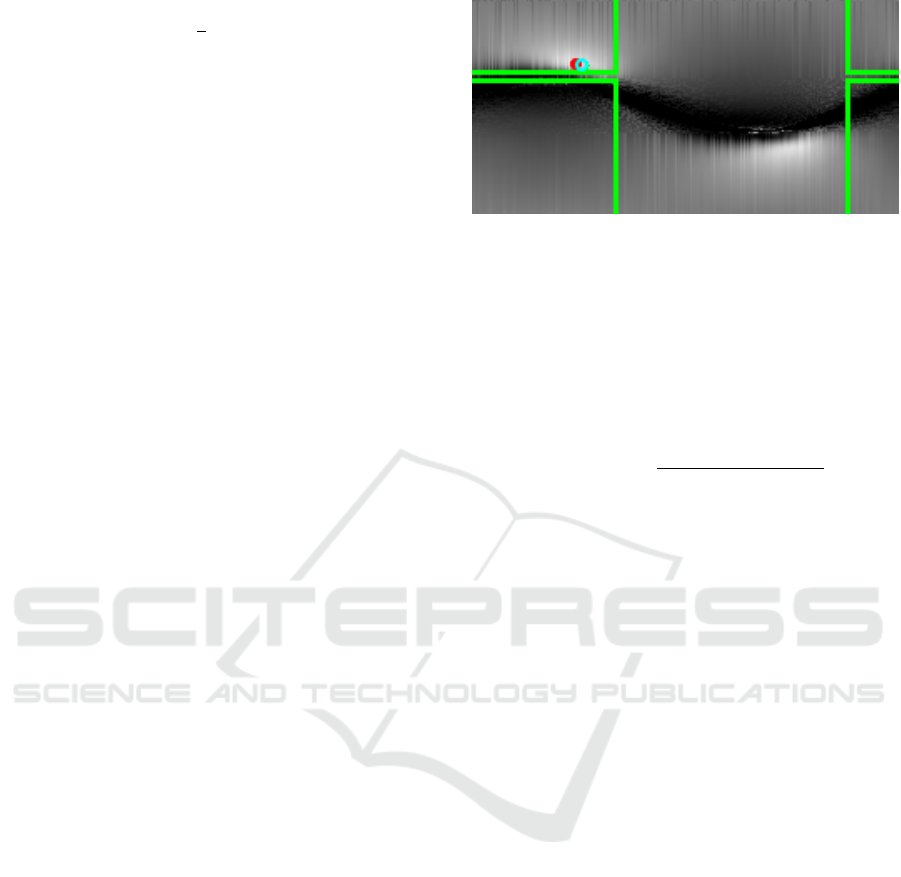
Figure 2: Measurement surface of an experiment on real

data. The horizontal and vertical axis are the u, and v pa-

rameters, respectively. Cropped green rectangle are the area

deﬁned by the visibility constraint. Cropping is because of

the periodicity of the parameter space. Red and blue dots

are the global optimum determined by exhaustive search on

the full parameter space and the result of PSO, respectively.

number n

opt

as the search area shrinks (see section

3.2.1).

opt

= min





100

rect[min

u,v

, max

u,v

]



(13)

where

rect

is the area of the rectangle. This gave a

mild drop in running times, without losing accuracy.

Fig. 2 shows the measurement surface of an ex-

periment on real data. The horizontal and vertical axis

are parameters u, and v, respectively. Therefore, the

coordinates of top-left, and bottom-right points de-

note [0,0]

, and [2π,π]

, respectively. The cropped

green rectangle encapsulates the area deﬁned by the

visibility constraint. (Note the periodicity of the pa-

rameter space.) Red and blue dots are the global op-

timum determined by ES on the full parameter space

and the result of PSO, respectively. As it is expected,

the remaining search space contains the global opti-

mum. The resulting coordinate pair (blue dot) are

close to the expected one. There is a gap of invalid

(black) values in the middle, which is caused by the

constraints based on Eq. 12. Thereby, several val-

ues are simply ommited, which are represented by

similarity value 0. It can be seen, that the similarity

function is not convex due to the two peaks, and the

black constant region. Remark that our preliminary

experiments showed, that the ommited area also con-

tains high peaks, even so, the surface normal is invalid

there. Unfortunately, gradient descent is not a valid

solution for that problem, since the region encapsu-

lated by the visibility rectangle is not convex either.

4 TESTS

In this section we show that the proposed method

works well on semi-synthesized tests and real-world

VISAPP 2016 - International Conference on Computer Vision Theory and Applications

692

photos. Unless otherwise noted we used s = 70 for

2D patch sizes and σ =

for the Gaussian.

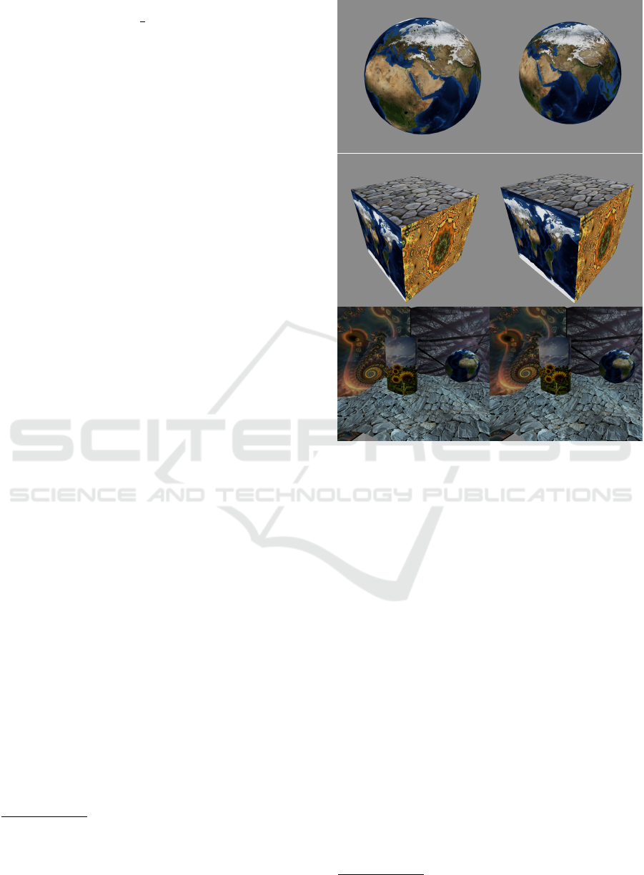
4.1 Semi-synthesized Tests

Three type of well-textured synthetic scenes were

generated using Processing

: a unit sphere, a unit-

edge cube, and a complex scene. This scene consists

of two perpedicual planes, a cylinder, a sphere, and

a parametric surface. The intrinsic and the extrin-

sic parameters of the camera setups were known, as

well. We took screenshots of the scenes from differ-

ent viewpoints (see Fig. 3). In order to get feature

points, ASIFT feature matcher (Yu and Morel, 2009)

was applied. Then the proposed algorithm ran on each

point pair, in order to compute the surﬂets. The com-

puted error value is the average angular error of the

surface normals w.r.t. the ground truth ones.

Fig. 3 shows two views of “Sphere”, “Cube”, and

“Complex” test scenes.

For the sake of comparison,

we reconstructed the scene by PMVS (Furukawa and

Ponce, 2010) and the standard LS Plane (Hoppe et al.,

1992) algorithm was also applied, in order to estimate

surface normals from the raw point clouds.

In Table 1, four methods are evaluated: ITPE-

PSO, ITPE-ES, PMVS and LS Plane. It is visible that

our method (ITPE-PSO) achieves smaller than 6.5°

average angular error in every test case, and the me-

dian errors are also below 3.5°, 1.2°, and 3.5° for the

sphere, cube and complex scenes, respectively. This

means that in the case of the cube, half of the surface

normals are closer to the ground truth than 1.2°. It is

also shown that the results of the rival methods are ap-

proximately three, ten, and two times less accurate in

the three cases. In Table 2 processing times of ITPE-

PSO, ITPE-ES methods are shown. It is apparent that

ITPE-PSO gives almost the same results as ITPE-ES

(Table 1), even so it is is ten times faster (Table 2).

Synthesized tests show that the proposed algo-

rithm works well and its processing time is low. As

it can be seen in Table 1, the average angular error of

the estimated surface normal in sphere and cube tests

are 5.5° and 2.09°, respectively. This result is consid-

erable given per-point estimation.

4.1.1 Free-form Surfaces

The proposed algorithm is also applied to real pho-

tos we acquired by handheld cameras. We assume

https://processing.org/

3D reconstruction results are visualized in (Cignoni

et al., 2008). The test environment was a notebook with

an Intel(R) Core(TM) i7-3610QM CPU at 2.30GHz, with 8

cores and 8192MB of RAM.

Figure 3: Input stereo image pairs of the synthetic tests.

The ﬁrst, second and third rows show the input of test cases

“Sphere”, “Cube” and “Complex”, respectively.

that the intrinsic parameters are known. The relative

pose of the setup is recovered (Bradski et al., 2000)

from the Essential matrix, which is calculated from

the Fundamental matrix (F). F is estimated from cor-

responding ASIFT (Morel and Yu, 2009) point pairs.

Then ITPE-PSO method was applied to each point

pair. In order to validate the results, we performed

Poisson reconstruction (Kazhdan et al., 2006) of the

3D point clouds and the related normals.

Fig. 4 consists of photos of a textured bear (honey

bottle) with high curvatures. The ﬁrst two images are

the stereo image pair that was used during the normal

reconstruction. The last two images are two views of

the reconstructed surface. As it can be seen our algo-

rithm accurately follows the shape of the observed ob-

ject even though the estimation is point-wise, it takes

only the local features into consideration. The quality

of the reconstruction is the best observed around the

nose of the bear from a side-wise view. The result is

much better than MeshLab LS Plane implementation

even though the curvature is high.

For the sake of comparison, we used PMVS

(Fu-

http://ccwu.me/vsfm (application available online)

A Novel Technique for Point-wise Surface Normal Estimation

693

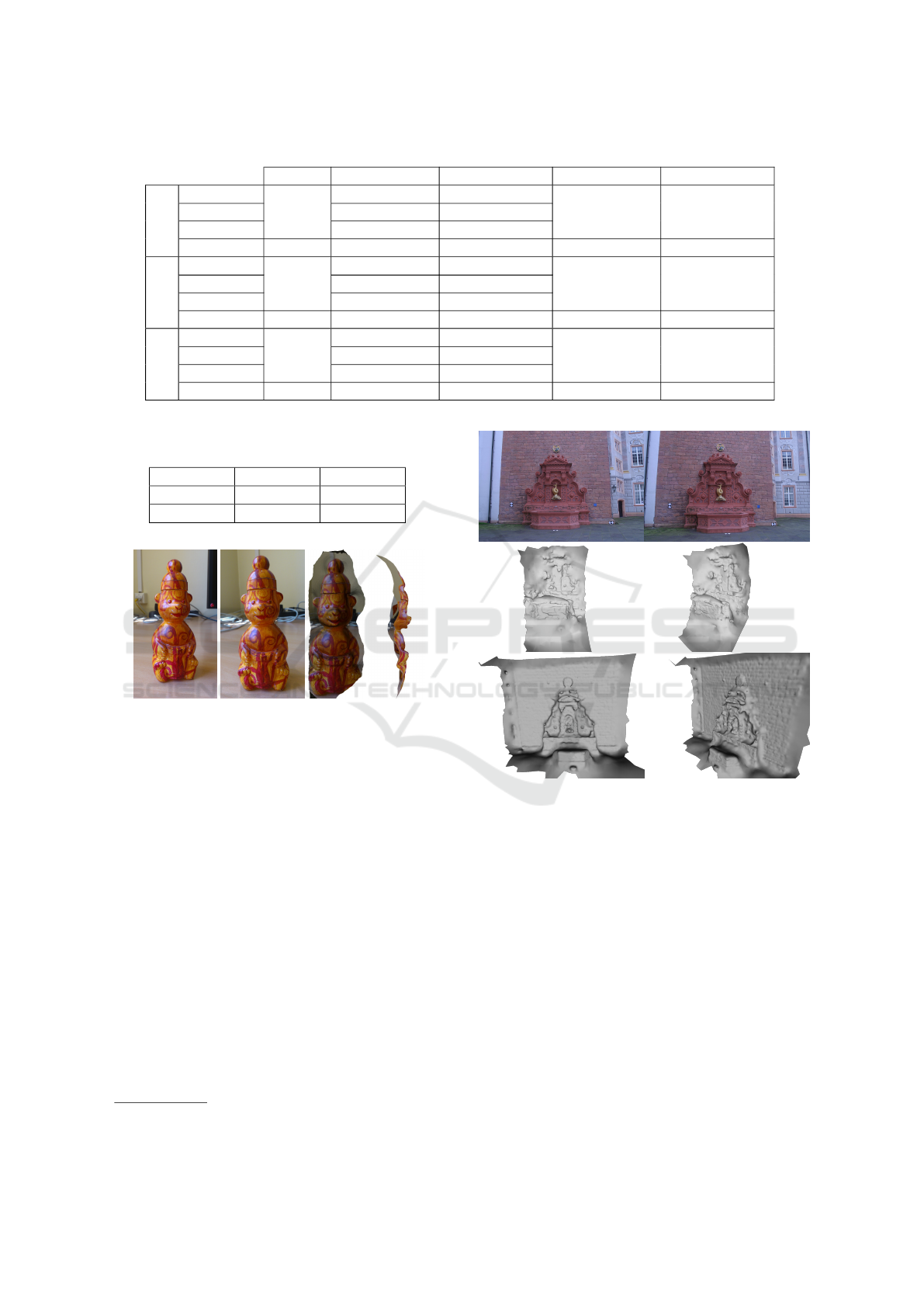
Table 1: Estimation results with σ = 50 and window size is 100 px.

#points Avg. ang. err. Med. ang. err. Avg. dist. err. Med. dist. err.

Sphere

ITPE-PSO

9492

5.5225° 3.4042°

0.0310 0.0321ITPE-ES 5.5021° 3.3994°

LS Plane 30.5298° 22.1780°

PMVS 12658 16.6978° 9.4666° 0.0416 0.0433

Cube

ITPE-PSO

9960

2.0883° 1.1481°

0.0581 0.0585ITPE-ES 2.0767° 1.1352°

LS Plane 25.1969° 29.6932°

PMVS 13376 24.6775° 21.9029° 0.0908 0.0907

Complex

ITPE-PSO

15343

6.3756° 3.4440°

0.0181 0.0158ITPE-ES 6.3461° 3.4280°

LS Plane 22.0623° 11.0703°

PMVS 47114 12.0152° 9.7374° 0.0272 0.0283

Table 2: Per-point processing times of ITPE-PSO and

ITPE-ES methods (window size is 100 px).

Sphere Cube

ITPE-PSO 0.0265 sec 0.0283 sec

ITPE-ES 0.1884 sec 0.2035 sec

Figure 4: The ﬁrst two images is the stereo image pair taken

from the observed honey bear. The last two images are

views of the Poisson reconstruction applied to the resulting

oriented point cloud, respectively.

rukawa and Ponce, 2010) to reconstruct the scene us-

ing an image pair from dataset fountain-P11

. Then

the same stereo pair was processed by our method, as

well. Surﬂets were estimated in both cases, then Pois-

son reconstruction was applied to the resulting point

clouds using the same parameter setup.

Fig. 5 shows Poisson reconstructions applied to

the output of the methods. The ﬁrst row consists of

the stereo image pair which was used. The second and

third rows consist of the results of PMVS and ITPE

from different viewpoints, respectively. It is obvious

that our method gives much more sophisticated result

using the same parameter setup. Remark that PMVS

implements dense reconstruction and surface propa-

gation, as well, by contrast our proposed method does

not. Even so our results approximate the original sur-

face signiﬁcantly better using the same input.

http://cvlabwww.epﬂ.ch/data/multiview/

Figure 5: The ﬁrst, second and the third rows consist of

stereo image pairs taken from Fountain dataset, Poisson re-

construction applied on the result of PMVS from two view-

points and the reconstruction of ITPE-PSO from two view-

points, respectively.

5 CONCLUSION

This paper was motivated by the imprecision of the

normal vectors estimated by state-of-the-art recon-

struction algorithms. As it is shown the proposed

method can estimate more accurate tangent planes

than the rival algorithms and the same accuracy of

the point locations. The beneﬁt of using afﬁne trans-

formation instead homography is that it makes the

proposed theory applicable to general camera model.

Moreover, no image undistortion needed.

Compared to other methods (Furukawa and

VISAPP 2016 - International Conference on Computer Vision Theory and Applications

694

Ponce, 2010; Hoppe et al., 1992; Vu et al., 2012;

Megyesi et al., 2006; Lhuillier and Quan, 2005) the

novelty of the proposed algorithm is threefold:

1. As a theoretical contribution: the search space

is narrowed by novel epipolar and geometry-based

constraints. It is mathematically ensured that the new

search space still contains the optimal solution. These

proposed constraints can be extended to multi-view

reconstruction straightforwardly.

2. Particle Swarm Optimization makes global op-

timum available with suitable speed. The proposed

method is well-parallelizable, with its per-point pro-

cessing time is below 0.03 sec. Therefore, a good

GPU implementation could make it real-time capable.

3. It is applicable to various types of cameras,

such as the perspective and omni-directional ones.

We believe that the proposed method is a powerful

tool to be used for sparse reconstruction and provides

a good base for future multiple-view methods.

REFERENCES

Barath, D., Molnar, J., and Hajder, L. (2015). Optimal Sur-

face Normal from Afﬁne Transformation. In VISAPP

2015, pages 305–316.

Bradski, G. et al. (2000). The OpenCV library. Dr. Dobb’s

Journal of Software Tools, 25(11):120–126.

Cagnoni, S. (2008). Evolutionary computer vision: a taxo-

nomic tutorial. In HIS’08. Eighth International Con-

ference on, pages 1–6. IEEE.

Cignoni, P., Corsini, M., and Ranzuglia, G. (2008). Mesh-

lab: an open-source 3d mesh processing system.

Ercim news, 73:45–46.

Faugeras, O. and Keriven, R. (2002). Variational princi-

ples, surface evolution, pde’s, level set methods and

the stereo problem. IEEE.

Faugeras, O. and Lustman, F. (1988). Motion and struc-

ture from motion in a piecewise planar environment.

Technical Report RR-0856, INRIA.

Furukawa, Y. and Ponce, J. (2010). Accurate, dense,

and robust multiview stereopsis. Pattern Analy-

sis and Machine Intelligence, IEEE Transactions on,

32(8):1362–1376.

Habbecke, M. and Kobbelt, L. (2006). Iterative multi-view

plane ﬁtting. In Int. Fall Workshop of Vision, Model-

ing, and Visualization, pages 73–80.

Habbecke, M. and Kobbelt, L. (2007). A surface-growing

approach to multi-view stereo reconstruction. In

CVPR’07. IEEE Conference on, pages 1–8. IEEE.

Hoppe, H., DeRose, T., Duchamp, T., McDonald, J., and

Stuetzle, W. (1992). Surface reconstruction from un-

organized points, volume 26. ACM.

Kazhdan, M., Bolitho, M., and Hoppe, H. (2006). Pois-

son surface reconstruction. In Proceedings of the

fourth Eurographics symposium on Geometry pro-

cessing, volume 7.

Kennedy, J. (2010). Particle swarm optimization. In Ency-

clopedia of Machine Learning, pages 760–766.

Lhuillier, M. and Quan, L. (2005). A quasi-dense ap-

proach to surface reconstruction from uncalibrated

images. Pattern Analysis and Machine Intelligence,

IEEE Transactions on, 27(3):418–433.

Martin, J. and Crowley, J. L. (1995). Comparison of cor-

relation techniques. In International Conference on

Intelligent Autonmous Systems, Karlsruhe (Germany),

pages 86–93.

Megyesi, Z., K

os, G., and Chetverikov, D. (2006). Sur-

face normal aided dense reconstruction from images.

In Proceedings of Computer Vision Winter Workshop.

Telc:[sn]. Citeseer.

Moln

ar, J. and Chetverikov, D. (2014). Quadratic transfor-

mation for planar mapping of implicit surfaces. Jour-

nal of mathematical imaging and vision, 48(1):176–

184.

Morel, J.-M. and Yu, G. (2009). Asift: A new framework for

fully afﬁne invariant image comparison. SIAM Jour-

nal on Imaging Sciences, 2(2):438–469.

Pons, J.-P., Keriven, R., and Faugeras, O. (2007). Multi-

view stereo reconstruction and scene ﬂow estimation

with a global image-based matching score. Interna-

tional Journal of Computer Vision, 72(2):179–193.

Shi, Y. and Eberhart, R. (1998). A modiﬁed particle swarm

optimizer. In Evolutionary Computation Proceedings,

1998. IEEE World Congress on Computational Intel-

ligence., The 1998 IEEE International Conference on,

pages 69–73. IEEE.

Strecha, C., Fransens, R., and Van Gool, L. (2006).

Combined depth and outlier estimation in multi-view

stereo. In CVPR’06 IEEE Computer Society Confer-

ence on, volume 2, pages 2394–2401. IEEE.

Vu, H.-H., Labatut, P., Pons, J.-P., and Keriven, R. (2012).

High accuracy and visibility-consistent dense multi-

view stereo. Pattern Analysis and Machine Intelli-

gence, IEEE Transactions on, 34(5):889–901.

Yu, G. and Morel, J.-M. (2009). A fully afﬁne invariant im-

age comparison method. In ICASSP 2009. IEEE In-

ternational Conference on, pages 1597–1600. IEEE.

Zaharescu, A., Boyer, E., and Horaud, R. (2007). Trans-

formesh: a topology-adaptive mesh-based approach

to surface evolution. In ACCV’07, pages 166–175.

Springer.

A Novel Technique for Point-wise Surface Normal Estimation

695