Occluding Edges Soft Shadows

A New Approach for Realistic Shadows using Occluding Edges

Christian Liwai Reimann and Bernd Dreier

Department of Computer Science, Kempten University of Applied Sciences, Bahnhofstr. 64, 87439 Kempten, Germany

Keywords:

Soft Shadow, Linear Light.

Abstract:

In this paper, a new algorithm to render soft shadows in real time applications is introduced, namely the

Occluding Edges Soft Shadow algorithm (short OESS). The algorithm approximates the shadow cast from

linear lights by ﬁnding the outlines of an occluding object (Occluding Edges) and considering these in a

fragment’s illumination. The method is based on the shadow mapping technique, whereby its capability of

rendering the shadow at an interactive rate does not depend on the complexity of the scene. The paper supplies

an overview for several methods to produce shadows and soft shadows in real time computer graphics, a

detailed description of the newly developed algorithm, and a section with results and future possibilities for

improvements.

1 PREVIOUS WORK

The illustration of hard shadows in computer games

has been common for decades. However, the pro-

duction of realistic soft shadows in real-time appli-

cations remains a difﬁcult task. In the area of real-

time shadowing, there are two basic algorithms which

are commonly used. The ”shadow mapping” algo-

rithm is a pixel based solution introduced in ”cast-

ing curved shadows on curved surfaces” by Lance

Williams (Williams, 1978). The second commonly

used technique is the ”shadow volume” method where

the shadow is considered as a volumetric object ex-

tracted out of the geometry of a scene. Both methods

exclusively produce hard shadows. Nonetheless, the

majority of algorithms for soft shadows can be con-

sidered as an extension of one or the other. This sec-

tion is a brief summary of several existing soft shadow

algorithms for real-time applications, extending the

shadow mapping technique.

In 1996, Michael Herf and Paul S. Heckbert, de-

scribed a relatively straightforwarsectiond algorithm

which renders high quality soft shadows for static

scenes (Heckbert and Herf, 1997). To produce

shadow, a set of point light samples is placed on a

grid in the area of the light source. Each light sam-

ple is used to render a shadow map. These shadow

maps are combined to so called ”radiance textures”.

When the static scene gets displayed in real time, the

radiance textures are mapped to the shadow receiving

objects.

Percentage closer ﬁltering is an approach to anti-

alias shadow maps, that was introduced in ”Rendering

Antialiased Shadows with Depth Maps” by William

T. Reeves et al. (Reeves et al., 1987). The method

can produce a smooth transition between shadowed

and non-shadowed areas, where the size of the tran-

sition area can be inﬂuenced by setting the size of

the ﬁltering area. Randima Fernando’s Percentage

Closer Soft Shadow algorithm (short PCSS) uses this

ability to automatically adapt the penumbra size to

generate more realistic shadows (Fernando, 2005).

The algorithm consults randomly chosen pixels of the

shadow map, near the lighted fragment. It is calcu-

lated whether a pixel belongs to a occluder or not. To

obtain the penumbra size, the averaged depth of the

occluding pixels is set in relevance with the fragments

distance to the light source. Only a single point light

sample is needed.

Another algorithm that works with a single light

sample is presented by Gregory S. Johnson et al. in

2009 (Johnson et al., 2009). The method, Soft Irreg-

ular Shadow Mapping, approximates soft shadows by

backprojecting the silhouette of the occluding object

and the receiving point to the light source. This pro-

jection is then used to calculate the portion of the light

seen by the receiving point.

Many light sources in the real world are elongated,

for instance ﬂuorescent tubes. For such light sources

we don’t necessarily need area light algorithms. Elon-

Reimann, C. and Dreier, B.

Occluding Edges Soft Shadows - A New Approach for Realistic Shadows using Occluding Edges.

DOI: 10.5220/0005777701770184

In Proceedings of the 11th Joint Conference on Computer Vision, Imaging and Computer Graphics Theory and Applications (VISIGRAPP 2016) - Volume 1: GRAPP, pages 179-186

ISBN: 978-989-758-175-5

179

gated light sources can also be approximated with al-

gorithms for linear light sources, which may require

less computing resources.

In 2000, Heidrich et al. introduce the soft shadow

maps algorithm (Heidrich et al., 2000) which approx-

imates the shadow of a linear light, by placing a sam-

ple (point light source) on each end point of the light

source. Both samples have an individual interval of

occluded area on the receiver. In other words, some

areas on the surface of the receiver are seen by both

point light sources. Other areas can only be seen by a

single sample, and some areas aren’t seen at all. The

algorithm approximates soft shadow, by applying a

simple linear blend in those areas of the scene, which

are only visible to a single light sample.

2 APPLIED CONCEPT

The share of the extended light which is seen by a

fragment, deﬁnes how much a fragment is lighted.

The OESS-Concept is developed to estimate this

value by determining the ”occluding edge” of the

shadow casting object. The ”occluding edge” is the

silhouette of the occluding object seen from the point

of view of a fragment lying in the penumbra. Figure 1

shows how the occluding edge E can be used to sep-

arate the light into two sectors: Sector l illuminating

fragment F, and sector o which is being occluded. A

is the point where the light source switches from seen

to not seen by the fragment. The ratio between l and

Figure 1: The extrapolated line between a fragment and an

occluding edge, separates the light source in a seen and a

non-seen sector.

o can then be used to calculate the lighting value of

any fragment.

The problem of how to shade a fragment can

therefore be broken down to the challenge of ﬁnding

the occluding edge of the shadow casting object. As

mentioned above, occluding edges are the silhouettes

of the occluding object from the perspective of a

fragment in the penumbra. But it is not practicable

to render the scene from the point of view of every

relevant fragment. So the occluding edges have to

be found by using the rendering results of point light

samples on the extended light source. The idea of

using the silhouette of the occluder to determine

penumbra in the pixel space of a shadow map, was

already applied in the soft irregular shadow mapping

method (Johnson et al., 2009), but the further steps of

our approach are different.

Transferring the Concept into Three-Dimensional-

Space: The Occluding Edges Soft Shadow algorithm

is a process of steps that calculate soft shadows. Some

of these steps are explained and implemented in two

dimensional space. To be able to apply them in a three

dimensional scene, the scene has to be transferred to

two dimensions. This can be done by following the

concept of Heidrich et al.:

”Consider the intersection of the scene with

a plane containing the light source. If we

can solve the visibility problem for all such

planes, i.e. for the whole bundle of planes

having the light source as a common line, then

we know the visibility of the light source for

all 3D-points in the scene.” (Heidrich et al.,

2000)

3 OESS PIPELINE STEPS

This section presents the OESS algorithm’s functional

principle, which is a series of steps (pipeline). The

algorithm is meant to work with only two point light

samples, which are placed on each end of a linear light

that is to be approximated. This set of two point sam-

ples (sample left, sample right) is what will represent

our light in the rest of the section.

Point light samples on an extended light source

each have a somewhat different perspective on a

scene. Some parts of the scene behind an occluder are

blocked for one light sample and not for another. For

twice sampled linear lights speciﬁcally, this means

that the shadow map of the left sample will always

contain more information about the scene left to an

occluder and vice versa. The sum of information con-

tained by both shadow maps, cannot be simply rep-

resented on a single map. To avoid loss of data, the

output of the ﬁrst three pipeline steps is produced for

both samples separately, and only at the end of step

four, the two data threads are combined to a single

value of shadow. Figure 2 shows the rough pipeline

of the newly introduced algorithm.

3.1 Step 1: Prerendering the Scene

Similar to most shadow map based soft shadow

algorithms, the OESS starts by rendering a standard

GRAPP 2016 - International Conference on Computer Graphics Theory and Applications

180

Figure 2: The rough pipeline of the OESS with the data required and produced in the individual steps.

shadow map from the point of view of each point

light sample. Simultaneously, an extra layer of

each shadow map, a so called ”metadata map”, is

generated.

Metadata Map: In the actual rendering step of

the shadow mapping algorithm, each fragment is as-

signed a pixel of the shadow map. Similarly, in the

OESS the pixels of the shadow maps of the point light

samples are mapped into each other’s pixel spaces to

ﬁnd out which pixels contain information about the

same part of the scene (corresponding pixels).

The meta data map holds additional information

about each pixel of the shadow map, other than the

depth. The coordinates of the corresponding pixels

are one out of two components of the map. The other

component is the fragment’s tilt to the light sample.

3.2 Step 2: Determining the Occluding

Edges

In this step of the pipeline, the occluding edges are

computed within a ”compute shader”. We use this

type of shader stage to prevent having to render the

scene again. Not the scene itself, but the shadow and

the meta data maps are used to determine the occlud-

ing edges.

From the perspective of a fragment, occluding edges

are the silhouette edges of occluders. But as already

mentioned, it is not feasible to render the scene from

every fragment in the penumbra region, to determine

the occluding edges in real-time. In the scope of this

work no solution was found to determine the exact

and physical correct occluding edges for every frag-

ment in an acceptable time. With the intent to com-

pute nearly realistic occluding edges by using the ren-

dering results of the two light samples, the two fol-

lowing strategies were developed. The basic idea of

the strategies is to ﬁnd the starting point of a penum-

bra region, and to pretend that this point was the oc-

cluding edge for the whole penumbra.

Each of the strategies have speciﬁc issues, but the

methods can be combined to utilize their advantages

and to achieve a consistent detection of the occluding

edges.

Strategy 1 - Tilt of Fragments: In the previous

pipeline step, all fragments that resulted to pixels in

the shadow map of the right light sample, are front

facing the sample (assuming solid objects). Conse-

quently, fragments which are seen by the left light

sample and back face the right light sample, are not

visible to the right side of the linear light source. They

are lying in the penumbra. We can determine whether

a fragment in Step 1 was back or front facing any

light sample, by considering the tilt value of the cor-

responding pixel in the metadata map.

A pixel p

in the left shadow map is deﬁned as an

occluding edge, if its origin fragment was front fac-

ing the right sample, but the origin fragment of the

left neighboring pixel of p

was back facing the right

sample. The detection of the occluding edges on the

right side of an occluder works analogously with the

right shadow map.

Unfortunately, this strategy only works for

occluding surfaces, that actually have a penumbra

region right next to the occluding edge.

Strategy 2 - Location of Corresponding Pixels:

Considering p

as a pixel of the 1D-shadow map of

one light sample, p

as its neighbor with a bigger

index, and c

as their corresponding pixels in the

shadow map of the other light sample, then c

usually

has a bigger index then c

. If the index of c

is smaller

then the one of c

, p

is lying in the penumbra. We

can now use a third pixel p

, the next neighbor of p

and its corresponding pixel c3, to check if p

is the

ﬁrst pixel of the penumbra. p

is the ﬁrst pixel in the

penumbra, if c

and c3 have a smaller index then c

And, if p

is the ﬁrst pixel of the penumbra region,

then p

is an occluding edge.

This strategy works for hard edges, but if the edge

is rather soft, the corresponding pixel values in the

area around the soft edge, differ only minimally. The

position of the detected occluding edge is then highly

inﬂuenced by numerical inaccuracies.

3.3 Step 3: Outreaching the Occluding

Edge

Figure 3 shows the proﬁle of a scene in the upper

Occluding Edges Soft Shadows - A New Approach for Realistic Shadows using Occluding Edges

181

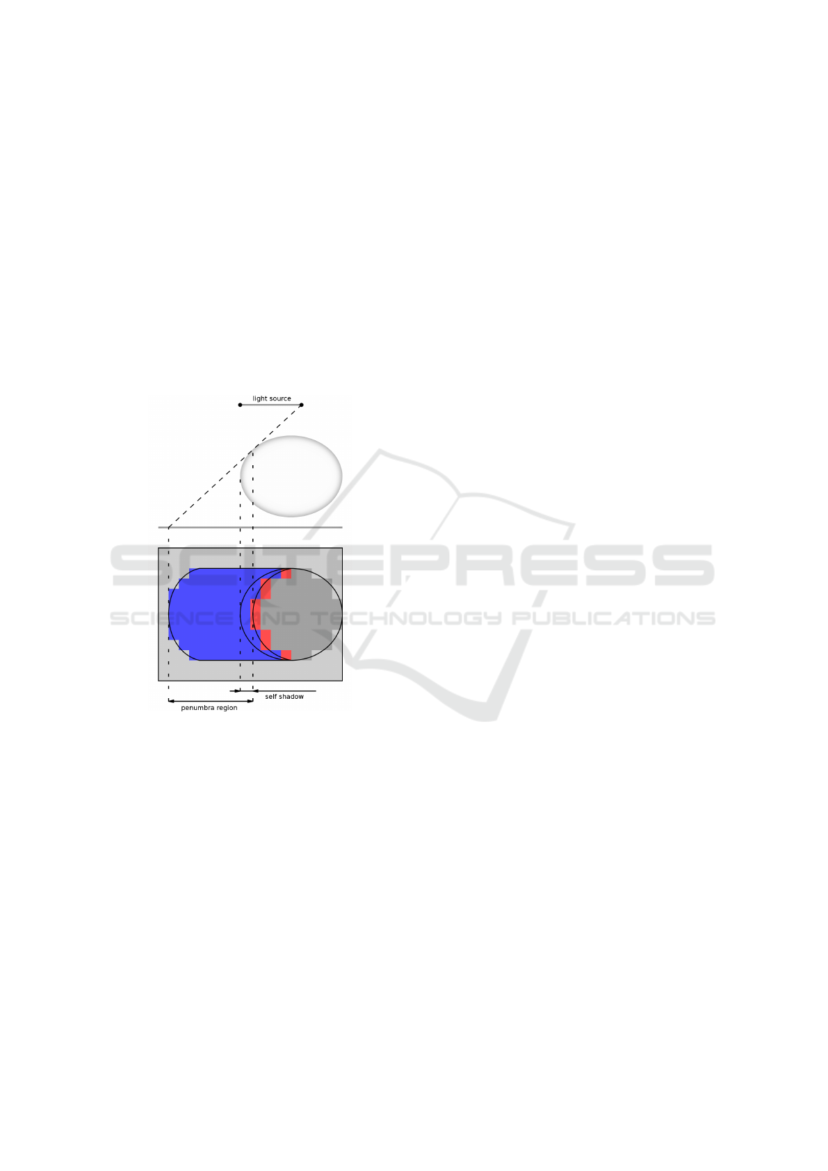
half, and the shadow map rendered from the left light

sample in the lower half. The dashed line that meets

the right light sample and is tangential to the round

occluder, shows which surfaces of the scene are vis-

ible to the right light sample. The point where this

line meets the receiving plane, is the end of the actual

penumbra region. The beginning of the penumbra re-

gion is at the point where the line touches the occlud-

ing object. The pixels of the illustrated shadow map

that lie in between this interval (penumbra region)

correspond to points in the scene, that are only vis-

ible to the left light sample. These pixels are marked

in blue. When the rendering for the screen is per-

formed, the blue pixels will be mapped to fragments

in the penumbra regions, that need an occluding edge

to calculate illumination.

Figure 3: Declaration of the penumbra region in the left

shadow map.

With the help of a compute shader we already de-

ﬁned, whether pixels of the shadow map are occlud-

ing edges or not (see Step 2). Therefore a shader ex-

ecution now knows if the pixel it treats matches to an

occluding edge. In Step 3, information from the oc-

cluding edge handling shader executions is passed to

the pixels in the penumbra region. I.e. in image 3

information, known within each red pixel has to be

transported to the blue pixels directly towards their

left. The data is stored in another layer of the shadow

map which is called ”occluding edge map”. The map

contains the coordinates of the occluding edge being

relevant for a pixel.

3.4 Step 4: Calculate the Lighting

So far we have rendered the scene from the per-

spective of the point light samples (shadow maps),

determined nearly realistic occluding edges, and have

written them into the occluding edges maps. In the

fourth step of the pipeline, the two shadow maps and

the two occluding edges maps are used to compute a

single value of illumination for each fragment in the

actual rendering. The illumination may be divided

into several substeps.

Substep 4.1 - Assigning Umbra and Penumbra:

Some pixels of the occluding edges map, hold data

about an occluding edge. These are mapped to the

corresponding parts of the scene, which are lying in

the penumbra. In a ﬁrst approach of assigning umbra

and penumbra region, only fragments with the same

depth as the respective pixel in a shadow map, were

considered to lie in the penumbra. Fragments not vis-

ible to any light sample were automatically declared

as part of the umbra.

The problem in doing so, is that the point we use

as occluding edge is only an approximation to the real

occluding edge of a particular fragment. A stark seam

between umbra and penumbra regions was the result.

By declaring all fragments with appropriate texture

coordinates as part of the penumbra, this abrupt tran-

sition can be avoided.

The assignment of penumbra status without

checking the visibility of a fragment however, also

has a disadvantage. Some fragments that lie beyond

a receiver, and should lie within absolute umbra, are

handled like a part of the penumbra only because of

their texture coordinates. This false classiﬁcation will

not be resolved within the realm of this paper.

Substep 4.2 - Direction to the Occluding Edge: The

task of ﬁnding the direction of the occluding edge, is

to compute the vector that points from a fragment F

towards its occluding edge E. All vectors that are

needed for the computation of this vector, are dis-

played in the upper half of ﬁgure 4.

L and R are the two point light samples. Point P

is the 3D-point that corresponds to the pixel with the

texture coordinates of fragment F in the left shadow

map. The 3D-coordinates of P can be computed with

the inverse projection matrix of the light source. The

vector

LE is read out of the occluding edge map.

is generated with the model-view-matrix of the left

light sample and the receiver-object. The lower half

of the image shows the section of the left shadow map

that contains the relevant pixels. The red colored pix-

els are those which are deﬁned as occluding edge.

GRAPP 2016 - International Conference on Computer Graphics Theory and Applications

182

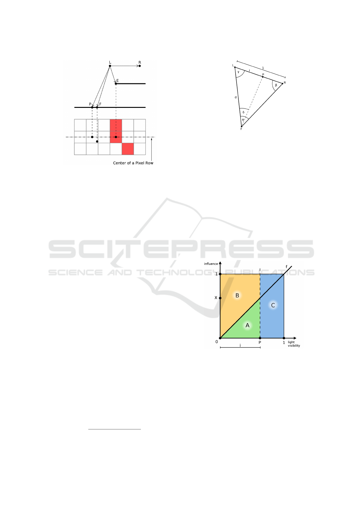
Figure 4: Determining the vector from a fragment F to-

wards its occluding edge E.

To complete the illumination properly, it is necessary

that the line deﬁned by F and

FE intersects the linear

light. This issue can be approached by using a frag-

ment’s texture coordinates to interpolate the positions

of two occluding edges. A fragment’s texture coordi-

nates lie between the center of two pixel rows. These

pixel rows have different occluding edges assigned.

We can interpolate the position of these occluding

edges linearly, so that in the occluding edges map,

the interpolated edge has the same y-coordinate as the

fragment. As the points share the same y-coordinate

in the map, they are lying on the same plane, together

with the light source.

The interpolation of the occluding edges as a

useful side effect, also solves the following problem.

If two fragments lie next to each other, but their tex-

ture coordinates correspond to different pixel rows,

they are assigned two different occluding edges. If

no interpolation was done the particular pixel rows

would become visible as stripes with a recognizable

difference in their gray scales (these stripes are prone

to be visually perceived over-contrasty due to the

Mach effect).

Substep 4.3 - Visibility of the Light Source: Fig-

ure 5 shows the triangle between the two point light

samples L and R and a fragment F that is located in

the penumbra region. Point P marks the end of the

luminiferous part i of the light. When considering the

entire size of the light as one, the size of i is equal to

the perceptual share of the seen light. d is the frag-

ment’s distance to the left light sample.

The formula for i is:

i =

sin(β) · sin(δ)

sin(α) · sin(π − δ− γ)

(1)

Figure 5: The luminiferous part of the light i and the mag-

nitudes needed for its deﬁnition.

After the seen sector (i) of the light is determined,

one must consider how strong this line segment of the

linear light is inﬂuenced by the individual point light

samples. I.e. a point on the linear light source which

is seen by a fragment has to impact the illumination

of the fragment. But the illumination model will only

be computed for the two point light samples, so we

have to interpolate the the results of those computa-

tions. The amount a single point on the light source is

inﬂuenced by the individual samples is described in

a linear function f in the OESS (see ﬁg. 6). In the

real world this function depends on the light emitting

consistency of the light source. By adjusting f the

shadow could be given more character. However, this

feature was not considered in the OESS.

Figure 6: Illustration of the distribution of impact on the

luminiferous line segment i.

Figure 6 visualizes how much inﬂuence on the seen

light segment i is distributed on the left versus the

righ light sample. Value i and point P refer to ﬁgure

5. We assume a fragment that lies in a penumbra

region left to an occluder and sees the light source

up to point P. The inﬂuence X of the right point

light on P, is determined by applying function f

on P. The left point light’s inﬂuence on P is given

by one minus X. The averaged inﬂuence-values for

all points of the luminiferous line segment can be

Occluding Edges Soft Shadows - A New Approach for Realistic Shadows using Occluding Edges

183

determined from the size of areas A and B, where the

size of A tells us how inﬂuential the right light sample

is in the illumination of the fragment and B holds

the inﬂuence-value of the left light sample. Area C

illustrates the part of the light source that is occluded.

Substep 4.4: Illumination Calculation and Merg-

ing: Substep 4.3 is performed for the penumbra left

of an occluder and right of an occluder separately. Yet

there are fragments which lie both in the left and the

right penumbra regions. Thus they get assigned two

values of inﬂuence for each point light sample. In

such a case, to perform the illumination of a frag-

ment, the values of inﬂuence of a light sample have

to be merged to a single value.

Finally, to illuminate a fragment, the illumination

models are performed for each point light sample.

The results are multiplied with the respective inﬂu-

ence value and summed up to the ultimate lighting

value of a fragment.

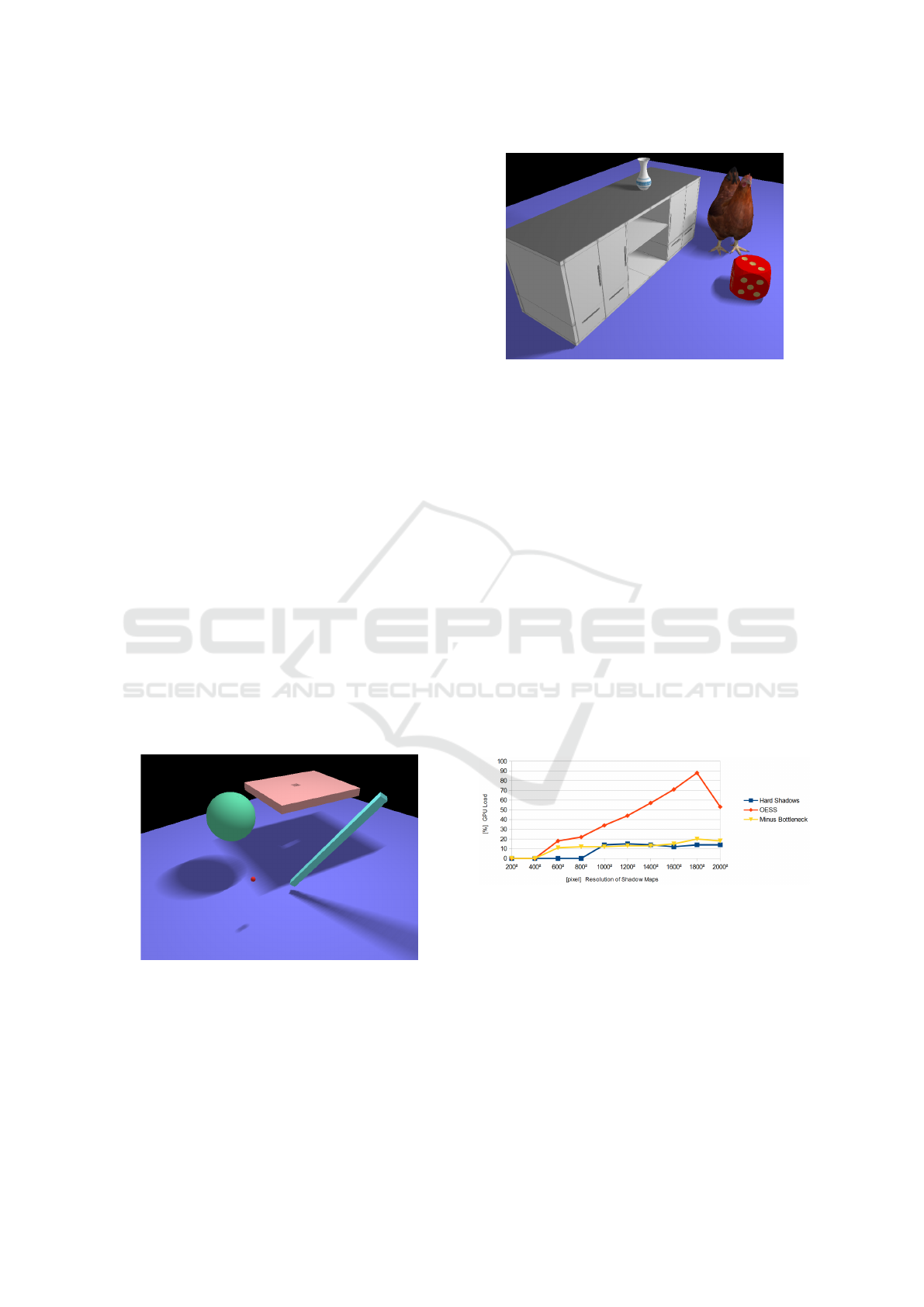
4 RESULTS AND OBSERVATIONS

Figures 7 and 8 show renderings where the OESS was

used to attain soft shadows. In ﬁgure 7, the algorithm

is tested on geometrical ﬁgures, each of which pro-

vide speciﬁc challenges. The scene presents shad-

owing results of small objects, objects with holes,

round surfaces, to the receiver parallel and non par-

allel edges as well as stark and smooth edges. The

shadows of the big sphere and the ﬂat cuboid are over-

lapping.

Figure 7: Rendering result of the OESS #1.

The scene in ﬁgure 8 shows the illumination of more

day to day objects. An aspect that becomes more ob-

vious in this scene, is self shadowing of objects.

Figure 8: Rendering result of the OESS #2.

5 PERFORMANCE

To test the performance on the GPU side (where the

major part of the OESS is processed), the OESS

was deployed to a PC with a ”Gigabyte HD 7950

WindForce” graphics card of AMD. The test was

performed using the scene of ﬁgure 8. The fol-

lowing three different implementations: ”Hard Shad-

ows” (two regular point light sources); ”OESS” (the

complete algorithm); ”Minus Bottleneck” (the OESS

without Step 3, which appeared to have large effect

on the runtime), were scope of the test. ”Minus Bot-

tleneck” runs the ”Outreaching the Occluding Edges”

step only in the ﬁrst frame, to be able to test the per-

formance of the rest of the algorithm separately.

The graph in ﬁgure 9 compares the percental GPU-

load of the three implementations depending on the

resolution of the shadow maps (and their layers).

Figure 9: Performance measured by the GPU load.

All tests were conducted at a stable framerate of 60

fps, except for the combination OESS / 2000

pixels,

where the GPU automatically adjusted the rate limit

to 30 fps (this explains the drop in the red curve). It

may also be noticed that the GPU load in the series

of measurements ”Hard Shadow” and ”Minus Bot-

tleneck” are hardly affected by the maps’ resolution

and almost stay constant. By contrast, the process-

ing expenditure over the entire OESS algorithm has

a distinctive growth with increasing resolution. Ap-

parently, the operation of writing the occluding edge

GRAPP 2016 - International Conference on Computer Graphics Theory and Applications

184

information to the pixels which map to penumbra re-

gion, is the only process in the algorithm that keeps it

from having a static load. This is due to the poor dis-

tribution of Step 3, where a small number of shader

executions writes to a much bigger number of pixels.

6 ARTIFACTS

The following sections describe problems of the

OESS that become visible in the rendered shad-

ows. Section ”Potential Future Improvements” then

presents some options how these artifacts could be

removed.

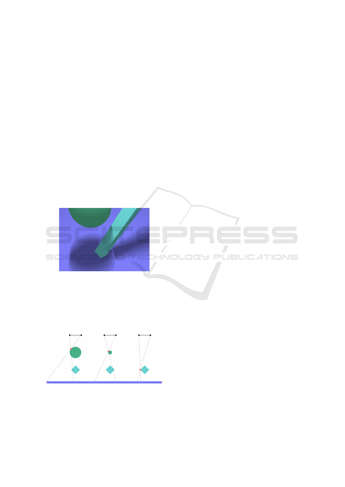
Object Alternation:

Figure 10 is a rendering output of the OESS. A sphere

and a pillar cast shadows on a ground object. When

looking at the edge of the sphere’s shadow, where the

shadow of the pillar becomes visible, we notice a hard

and abrupt transition. This unwanted hard transition

is the artifact called ”Object Alternation”.

Figure 10: Artifacts ”Object Alternation” and ”Spare Edge

Interpolation”.

To receive better understanding about why the ar-

tifact arises, ﬁgure 11 provides the sketch of three

cross-sections of the scene. These cross-sections rep-

resent the 2D scenes spanned by the pixel rows of the

shadow maps.

Figure 11: Reason of the ”Object Alternation” artifact.

The red point in each 2D scene is the determined

occluding edge. As the 2D scenes get close to end

of the sphere, the circle (cross-section of the sphere)

declines. This is illustrated in the ﬁrst two sections of

the image. The third section is the 2D scene, where

the circle ﬁnally disappears. Here the occluding edge

is found on the square, which means that the position

of the occluding edge strongly varies between the

second and the third image sections. This abrupt leap

of the occluding edge’s position causes the artifact.

Spare Edge Interpolation: Another artifact can be

found in ﬁgure 10. We notice stripes in the penumbra

region that are best visible in the shadow of the

pillar. To understand why these stripes appear, one

has to recall the circumstance that the occluding

edges are determined as pixels in the shadow maps

(Step 2: Determining the Occluding Edge). After

a pixel is determined to mach an occluding edge, a

three-dimensional position is calculated out of the

pixel’s center and is used as the position of an oc-

cluding edge. The resulting 3D-points are somewhat

a rasterized version of the silhouette of the occluding

object. In the fourth step of the OESS pipeline, the

occluding edges’ positions are interpolated to obtain

a smooth result. To trick the human eye, apparently

the interpolation must be carried out between more

than two positions.

Receiver Penetration: The assignment of penumbra

status without checking the visibility of a fragment

as described in Substep 4.1 ”Assigning Umbra and

Penumbra”, presents us another problem. Some frag-

ments that lie beyond a receiver, and should lie within

absolute umbra, are handled like a part of the penum-

bra only because of their texture coordinates.

7 POTENTIAL FUTURE

IMPROVEMENTS

Optimized Smoothing of Occluding Edges’ Posi-

tions: In the algorithm introduced in this paper, the

3D-positions of the occluding edges are interpolated

by simply mixing the coordinates of two neighboring

occluding edges (see ”Substep 4.2: Direction to the

Occluding Edge”). This Method is not ideal and

leads to the artifact described in section ”Spare Edge

Interpolation”. To patch this problem, it is important

to not only make the curve of the interpolated occlud-

ing edges’ positions constant and differentiable (for

instance with Bzier/Spline), but also to interpolate

between more than two edges.

Detecting Edges in the Penumbra: By detecting

additional edges located in the penumbra, a better

method of assigning the penumbra (see ”Assigning

Occluding Edges Soft Shadows - A New Approach for Realistic Shadows using Occluding Edges

185

Umbra and Penumbra” in Step 4 of the OESS

Pipeline) could be found, and the ”Receiver Penetra-

tion” artifact ﬁxed. Also, the ”Object Alternation”

problem is reduced as more edges are found.

However, ﬁnding additional edges in parts of the

scene, which are only visible to a single light sam-

ple, is quite a challenge. It’s conceivable that the

scene was re-rendered multiple times from the light

samples’ point of view, thereby ignoring fragments

which are already saved to a shadow map by setting

their depth value to ”inﬁnity”. Each rendering step

would produce a new layer of a shadow map. The

resulting maps would contain more information of

the penumbra than the conventional shadow maps,

which allows the determination of edges in this area.

Usage of Shadow Volume: Instead of using shadow

maps rendered by the point light samples, one could

ﬁgure out a way to implement shadow volumes to the

OESS algorithm. This would provide access to com-

pletely new opportunities. Instead of writing the posi-

tion of an occluding edge to a pixel, the color variable

of the shadow volumes’ faces could be used to store

the information of the edge. That way, the main leak

of performance would be avoided. Moreover, the de-

tection of occluding edges would not only be more

precise (due to not doing it in pixel space), but also

the edges in the penumbra areas would automatically

be determined. The ”Spare Edge Interpolation” arti-

fact would vanish as well.

8 CONCLUSION

In this paper we have presented a new strategy to com-

pute soft shadows, namely the OESS algorithm. It

was shown that the OESS can produce shadows of

high visible quality, even for object constellations in

which other methods fail. On the other hand, resulting

artifacts of the introduced technique were pointed out

and explained. In a performance test, it was demon-

strated that up to a shadow map resolution of 800

pixels, the new method is very time efﬁcient.

Because the described artifacts unfortunately oc-

cur quite commonly in scenes of average complexity,

the current version of the OESS algorithm would not

provide satisfying results for the majority of applica-

tions.

Nonetheless, the basic idea of the OESS (determine

occluding edges and consider them in the illumina-

tion calculation) seems to be a useful approach to ap-

proximate soft shadows. Several ideas to further de-

velop the algorithm procedure and resolve artifacts,

were discussed in section ”Potential Future Improve-

ments on the OESS”. Especially the employment of

the shadow volume algorithm looks quite promising

and could eventually make the OESS highly interest-

ing for 3D-applications.

REFERENCES

Fernando, R. (2005). Percentage-closer soft shadows. In

ACM SIGGRAPH 2005 Sketches, SIGGRAPH ’05,

New York, NY, USA. ACM.

Heckbert, P. S. and Herf, M. (1997). Simulating

soft shadows with graphics hardware. Technical

Report CMU-CS-97-104, Carnegie-Mellon Univer-

sity.Computer science. Pittsburgh (PA US), Pitts-

burgh.

Heidrich, W., Brabec, S., and Seidel, H.-P. (2000). Soft

shadow maps for linear lights. In P

eroche, B. and

Rushmeier, H., editors, Rendering Techniques 2000,

Proceedings of the 11th Eurographics Workshop on

Rendering, Springer Computer Science, pages 269–

280, Brno, Czech Republic. Eurographics, Springer.

Johnson, G. S., Hunt, W. A., Hux, A., Mark, W. R., Burns,

C. A., and Junkins, S. (2009). Soft irregular shadow

mapping: Fast, high-quality, and robust soft shadows.

In Proceedings of the 2009 Symposium on Interactive

3D Graphics and Games, I3D ’09, pages 57–66, New

York, NY, USA. ACM.

Reeves, W. T., Salesin, D. H., and Cook, R. L. (1987). Ren-

dering antialiased shadows with depth maps. SIG-

GRAPH Comput. Graph., 21(4):283–291.

Williams, L. (1978). Casting curved shadows on curved sur-

faces. SIGGRAPH Comput. Graph., 12(3):270–274.

GRAPP 2016 - International Conference on Computer Graphics Theory and Applications

186