Automatic and Generic Evaluation of Spatial and Temporal Errors in
Sport Motions
Marion Morel
1,2
, Richard Kulpa
1
, Anthony Sorel
1
, Catherine Achard
2
and Séverine Dubuisson
2
1
M2S Laboratory, Université Rennes 2, ENS Rennes, Avenue Robert Schuman, 35170 Bruz, France
2
Sorbonne Universités, UPMC Univ Paris 06, CNRS, UMR 7222, ISIR, F-75005, Paris, France
Keywords:
Dynamic Time Warping, Evaluation, Multidimensional Features, Synchrony, Motion Capture.
Abstract:
Automatically evaluating and quantifying the performance of a player is a complex task since the important
motion features to analyze depend on the type of performed action. But above all, this complexity is due
to the variability of morphologies and styles of both the experts who perform the reference motions and the
novices. Only based on a database of experts’ motions and no additional knowledge, we propose an innovative
2-level DTW (Dynamic Time Warping) approach to temporally and spatially align the motions and extract the
imperfections of the novice’s performance for each joints. In this study, we applied our method on tennis serve
but since it is automatic and morphology-independent, it can be applied to any individual motor performance.
1 INTRODUCTION
One of the key factors of sport performance is the mo-
tor control. The players must indeed accurately con-
trol their movements in space and time, for instance
by temporally synchronizing their limbs or by placing
a body part at a precise location, relative to their own
bodies or their surrounding environment. The pro-
gression of a novice player thus requires to identify
these spatiotemporal errors to correct them. This eval-
uation of a motion requires the expertise of a coach
due to the variability of correct performances. Each
expert has indeed his/her own way to perform the
movement depending on morphology, physical abil-
ities and style.
Some specific motions such as katas in karate
could be repeated and trained without the permanent
presence of a coach, at home for instance. How-
ever, an automatic evaluation system is then required
to identify and highlight the errors of the player to
help him make progress. Some tools are proposed
like the Golf Training System (Explanar Ltd, Manch-
ester, UK) or the PlaneSWING Training System (Por-
tugolfe Ltd, Bedfordshire, UK) in golf, but they are
dedicated to specific motions and to only a limited set
of features (for instance speed in a 2D plane). More-
over, only few studies are taking the morphology of
the players into account (Sorel et al., 2013).
The goal of this paper is to provide an efficient
and automatic morphology-independent and sport-
independent method to evaluate the motion of a player
by comparing it to a database containing the same mo-
tions performed by experts.
2 RELATED WORK
Being able to automatically evaluate the quality of
various actions requires to determine the kinematic
factors that are the core of a good performance for
each of these motions. For this reason, some authors
proposed to add knowledge to the motion evaluation
process to know in advance the features to analyze.
For instance, Burns et al. defined a set of rules that
characterizes some kata in karate, such as the linear
trajectory the kicking wrist must follow (Burns et al.,
2011). Komura et al. based their evaluation on the
minimization of the global movement since they con-
sidered that the defender can better counteract an at-
tack if he does not move too much just before the ac-
tion (Komura et al., 2006). Finally, Ward used sev-
eral intersegmental angles to compare several classi-
cal ballet techniques (Ward, 2012). These studies pro-
vide interesting results that are useful for evaluating
specific motions. However, our goal is to propose a
generic evaluation method that can automatically de-
544
Morel, M., Kulpa, R., Sorel, A., Achard, C. and Dubuisson, S.
Automatic and Generic Evaluation of Spatial and Temporal Errors in Sport Motions.
DOI: 10.5220/0005778505420551
In Proceedings of the 11th Joint Conference on Computer Vision, Imaging and Computer Graphics Theory and Applications (VISIGRAPP 2016) - Volume 3: VISAPP, pages 544-553
ISBN: 978-989-758-175-5
Copyright
c
 2016 by SCITEPRESS – Science and Technology Publications, Lda. All rights reserved

termine the important features of the expert motions
that are then used to evaluate the performance of a
new player.
Several authors have worked on this automatic ex-
traction of the relevant features of motions. It is in-
deed a prerequisite on other domains such as motion
recognition or motion retrieval in which these features
are both used 1) to group set of motions into cate-
gories of actions and 2) to differentiate these groups
of actions. For the first case, some authors have pro-
posed to identify common geometrical patterns of the
motions: by partitioning the 3D space with Cartesian
patches (Wang et al., 2012) or angular ones (Xia et al.,
2012), by simplifying the joints trajectories with lin-
ear regressions (Barnachon et al., 2013) or by using
pentagonal areas to represent the postures (Sakurai
et al., 2014). Some authors also worked on the re-
lation between the position of a joint relatively to a
plan defined by 3 other joints to give a semantic and
intuitive evaluation of the performed motion (Röder,
2006; Müller et al., 2005; Müller and Röder, 2006).
Finally, several authors tried to define morphology-
independent features to manage the morphology vari-
ability by normalizing the posture representation and
by extension the motion (Sie et al., 2014; Kulpa et al.,
2005; Shin et al., 2001). The goal of these studies
was to identify the similarity of motions while our is
to evaluate the difference between a motion and the
reference ones performed by experts. The motions
are thus supposed to be similar and our objective is
to quantify the errors between them and not to try to
ignore these small differences. For the second case,
some authors have computed the variance (Ofli et al.,
2012) or the entropy (Pazhoumand-Dar et al., 2015)
of each joint to discriminate the most informativefea-
tures characterizing the motion. The problem of such
approaches is that they lost some of the temporal in-
formation of the motion.
This temporal information is yet essential to eval-
uate motions and especially sports ones. The tempo-
rality of a movement is important for dance of course
but it also concerns all kinds of motions since the syn-
chronization of the limbs or the sequence of body mo-
tions are the key factors of a good technique and thus a
good performance. The temporal information is thus
essential at a global level but above all at the joints
level, highlighting the relative timing of the differ-
ent body parts of the player. Maes et al. proposed
to evaluate and train the basics of dance steps (Maes
et al., 2012). Since they considered that the dance
steps were very rhythmic, they based their analysis on
the music tempo of the dance. This case is however
very specific and only manages the synchronization
of the motion with an external and global tempo. To
take local synchronization into account, the temporal-
ity must be evaluated even when motions have differ-
ent lengths, different speeds and/or different rhythms.
To this end, some authors proposed to use Hidden
Markov Models (HMM) or Hidden Conditional Ran-
dom Field (HCRF) to encode time series as piecewise
stationary processes (Zhong and Ghosh, 2002; Kahol
et al., 2004; Sorel et al., 2013; Wang et al., 2006). In
our context, the time-varying features are trajectories
and are modeled as a state automaton in which each
state stands for a range of possible observation val-
ues of the feature while the transitions between states
can model time. The feature observation values and
the transitions between states are driven by probabili-
ties, which makes HMM very robust to spatiotempo-
ral variations. However, this approach gathers similar
postures together in a same state and the temporality
is only managed between these states that can repre-
sent a large part of the motion if at a period a joint
does not move a lot for instance.
To generically evaluate the synchrony of two mo-
tions, we need a more accurate method such as the
Dynamic Time Warping (Sakoe and Chiba, 1978).
Originally created for speech processing, DTW has
become a well-established method to account for tem-
poral variations in the comparison of related time se-
ries. Many studies havetried to upgrade the efficiency
of the DTW algorithm over the recent years depend-
ing on its application’s context (Keogh and Pazzani,
2001; Zhou and De La Torre Frade, 2009; Zhou and
de la Torre, 2015; Heloir et al., 2006; Gong et al.,
2014). In motion retrieval, DTW has then been used
by several authors to align the motion with some fea-
tures to determine the movement performed. Saku-
rai et al. for instance tried to evaluate a motion cap-
tured with the Microsoft Kinect by using pentagonal
areas defined by the body end-effector (Sakurai et al.,
2014). Pham et al. tried to compare surgery motions
by aligning trajectories of 3D sensors (Pham et al.,
2010). The problem of these studies is that the mo-
tion is simplified to manage the temporality and the
joint information are not preserved. In our approach,
we want to take temporal and spatial information into
account concurrently.
In this paper, we propose an efficient and au-
tomatic morphology-independent method based on
DTW to compare a motion performed by a player to a
database of experts’ motions in order to evaluate con-
currently the spatial and temporal relevant informa-
tion of the motion.
Automatic and Generic Evaluation of Spatial and Temporal Errors in Sport Motions
545

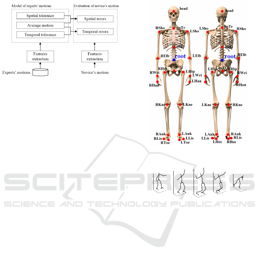
Figure 1: Global framework of the proposed approach.
3 METHODOLOGY
The purpose of this paper is to determine whether
a motion is correct or not and, if not, to determine
where and when it is badly performed. To this end,
we need to compare this motion to the reference ones,
the motions performed by experts. The reference can-
not indeed be only one motion because it is necessary
to take the variability of all experts performance into
account, all these motions are obviously considered as
correct ones. We thus first extract a reference model
of the correct motion from the database of experts’
movements (Section 3.2). We then compare the new
motion (for instance performed by a novice) to this
model to identify the spatial (Section 3.3.1) and/or
temporal errors (Section 3.3.2).
Our goal is to evaluate the motion of a novice
player in the context of individual sports. As a case
study, we applied our method on tennis serves. These
motions indeed present high spatial variabilities (con-
trary to codified motions such as kata in karate) and
require a strong coordination between body parts, to
achieve at the same time fast and accurate shots.
3.1 Database and Gesture Coding
To create the database, the tennis serves were cap-
tured with a Vicon MX-40 optical motion capture sys-
tem (Oxford Metrics Inc., Oxford, UK). The players
were equipped with 43 reflective markers placed on
anatomical landmarks to compute the trajectories of
the 25 joint centers as shown in Figure 2.
To create the database, we captured the tennis
serves of 9 experts (14-18 year old women) and 2
novice players. Each of them made 8 to 10 exam-
ples (or trials) leading to a database of 79 expert and
20 novice examples (see an example at different time
steps in Figure 3).
In order to be invariant to the initial position
Figure 2: The captured motion is represented by the trajec-
tories of these 25 joint centers.
−0.5
0
0.5
−0.8
−0.6
−0.4
−0.2
0
0.2
−1.5
−1
−0.5
0
0.5
1
x
y
z
−0.8
−0.6
−0.4
−0.2
0
0.2
0.4
−0.2
0
0.2
−1.5
−1
−0.5
0
0.5
1
1.5
x
y
z
−0.8
−0.6
−0.4
−0.2
0
0.2
−0.2
0
0.2
−1
−0.5
0
0.5
1
1.5
x
y
z
−0.5
0
0.5
−0.2
0
0.2
0.4
0.6
−1
−0.5
0
0.5
1
x
y
z
−0.5
0
0.5
−1
−0.5
0
0.5
−1.5
−1
−0.5
0
0.5
x
y
z
Figure 3: Skeletal representation of a captured tennis serve
at different time steps.
and orientation of the subject, the coordinate system
of each joint trajectories is centered on the root
position (see Figure 2) and oriented according to
the hips. Moreover, to decrease the influence of the
morphology, each joint coordinate is divided by the
distance between head and root joints as proposed by
Sie et al. in (Sie et al., 2014).
Let us now consider the following notations:
• A: number of joints (25 here).
• M
j
: number of time steps of the j
th
example.
• N
E
: number of expert examples (79) and N
N
:
number of novice examples (20).
• X
j
(t) = {x
a
j
(t),a = 1...A}, with
x
a
j
(t) = (x
a
j
(t),y
a
j
(t),z
a
j
(t)): trajectory of the a
th
joint and the j
th
example.
Thus, X
j
(t) is a 75-dimensional vector (25×3)
that encodes, at time t, the body posture (position
of all joints) while x
a
j
(t),a = 1...A only encodes
VISAPP 2016 - International Conference on Computer Vision Theory and Applications
546

the position of joint a at time t for the j
th
example
(3D vector).
3.2 Model of Experts’ Motions
The model of experts’ motions must at best repre-
sent all these motions with their variability to ensure
that an expert motion is never considered as incorrect.
One of the main problem to create such a model is
that each motion may have different durations. Mod-
els such as HMM or HCRF can overcome this prob-
lem but do not consider the temporality between the
limbs. They thus can consider as correct motions that
are properly executed but badly synchronized. An-
other approach could be to use a nearest neighbor
method but it becomes intractable when the number
of examples in the database increases. To overcome
these limitations and to ensure that our model per-
fectly represents all the experts’ motions with their
variability, we chose to model the serves with both
the average motion and the spatial and temporal tol-
erances between it and each serve of all experts. To
deal with the different motion durations, all examples
are temporally aligned with the longest example us-
ing a Dynamic Time Warping algorithm (DTW). Let
X
L
(t) be this longest example. This temporal align-
ment simultaneously considers all joints to ensure that
we model both the spatial features of the motion and
the temporality between joints.
3.2.1 Average Expert Trajectory
To determine the average motion of all experts, we
first made a global temporal alignment between each
expert example X
j
(t) and the longest example X
L
(t)
using DTW. To this end, we defined a distance matrix
that contains the similarity values between X
L
(t
1
) and
X
j
(t
2
), ∀t
1
∈ [ 0,M
L
− 1] and ∀t
2
∈ [ 0,M
j
− 1] where
M
L
and M
j
are the durations of trajectory L and j re-
spectively. These similarities are computed on both
each joint trajectory and its derivative, as suggested
in (Keogh and Pazzani, 2001):
d
1
L, j
(t
1
,t
2
) = kX
L
(t
1
) − X
j
(t
2
)k
2
d
2
L, j
(t
1
,t
2
) = k
˙
X
L
(t
1
) −
˙
X
j
(t
2
)k
2
d
L, j
(t
1
,t
2
) =
d
1
L, j
(t
1
,t
2
)
max
t
1
,t
2
d
1
L, j
(t
1
,t
2
)
+
d
2
L, j
(t
1
,t
2
)
max
t
1
,t
2
d
2
L, j
(t
1
,t
2
)
∀t
1
∈ {0...M
L
− 1},∀t
2
∈ {0...M
j
− 1}.
The cumulative distance matrix D
L, j
is then com-
puted from these similarities:
D
L, j
(t
1
,t
2
) = d
L, j
(t
1
,t
2
)+
min(D
L, j
(t
1
,t
2
− 1),D
L, j
(t
1
− 1,t
2
),D
L, j
(t
1
− 1,t
2
− 1)))
with D
L, j
(0,0) = d
L, j
(0,0), D
L, j
(t
1
,0) =
∑
t
1
−1
t=0
d
L, j
(t,0) and D
L, j
(0,t
2
) =
∑
t
2
−1
t=0
d
L, j
(0,t),
∀t
1
∈ {1...M
L
− 1},∀t
2
∈ {1...M
j
− 1}.
The distance between examples X
L
(t) and X
j
(t)
is then defined by D
L, j
(M
L
− 1,M
j
− 1). The mini-
mal path that goes from times (0,0) to times (M
L
−
1,M
j
− 1) of the two examples gives then their opti-
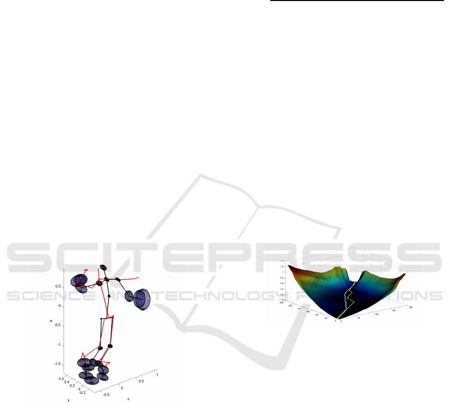
mal alignment as shown in Figure 4.
Figure 4: Cumulative distance matrix D
L, j
and the resulting
minimal path that align at best the two motions (in white).
This alignment method of each example X
j
(t) on
the longest one X
L
(t) is then applied to all examples
to compute their optimal path. This path provides the
T
L, j
(t) function that links each time t
1
of X
L
(t) to a
time T
j
(t
1
) of X
j
(t). Let us denote this path P
L, j
=
{(t
1
,T
L, j
(t
1
)),t
1
= 1...M
L
− 1}. Each example X
j
(t)
is then realigned according to the path P
L, j
to obtain
a new motion
˜
X
j
(t) with a duration of L time steps.
The average motion can then be simply computed like
this:
X
mean
(t) =
1
N
E
N
E
−1
∑
j=0
˜
X
j
(t) ∀t ∈ {1...M
L
− 1}
Let us recall that X
j
(t) contains the 3D trajectories
of all joints at time step t. The temporal alignment be-
tween trajectories is thus the same for the whole body,
ensuring to maintain the temporal coherency between
joints while being able to obtain the mean trajectory
of all joints: X
mean
(t) = {x
a
mean
(t),a = 1...A}.
Based on this mean motion that best represents all
expert examples, we now need to model the spatial
and temporal tolerances (deviations) that enclose all
the variability of experts’ performances.
3.2.2 Spatial Tolerance Modeling
To better evaluate and model the spatial tolerance of
the experts’ motions, we must be independent of tem-
poral errors, and do not allow bad synchronization
Automatic and Generic Evaluation of Spatial and Temporal Errors in Sport Motions
547

to influence the computation of spatial errors. We
thus consider each joint separately and align each of
them x
a
j
(t) to the mean joint trajectory x
a
mean
(t). To
this end, as described above, we compute the ele-
ments d
a
mean, j
(t
1
,t
2
) of the distance matrix between
joints as well as the cumulative distance matrix ele-
ments D
a
mean, j
(t
1
,t
2
). A specific path P
a
mean, j
is then
defined for each joint. It links each time t
1
of x
a
mean
(t)
to a time T
a
mean, j
(t
1
) of x
a
j
(t). Using these paths
P
a
mean, j
= {(t
1
,T
a
mean, j
(t
1
)),t
1
= 1...M
L
− 1}, new tra-
jectories
˜
x
a
j
(t) are obtained, that have the same dura-
tion (M
L
) but do not correspond to the same temporal
alignment. We can now compute the spatial tolerance,
for each joint and at each time step:
Σ
S
(t,a) = COV
j∈experts
{
˜
x
a
j
(t)}
where COV is the covariance matrix,
∀t ∈ {0...M
L
− 1},∀a ∈ {1...A}.
Each Σ
S
(t,a) is then a 3× 3 matrix that represents
the variations of position of the joint a, in the 3D co-
ordinate system (x, y, z) and at time t, that are allowed
around the mean 3D position to be still considered as
a correct position (a position that experts can have).
The spatial tolerance is illustrated for a specific time t
and all the joints a in Figure 5.
Figure 5: Spatial tolerance of the model of experts’ motions.
The black posture represents the average expert posture at
time t and the black spheres are the spatial tolerance of all
joints around this posture. The red posture is an example of
novice posture.
3.2.3 Temporal Tolerance Modeling
If the joints of experts are perfectly synchronized,
the alignments computed for each joint P
a
mean, j
=
{(t, T
a
mean, j
(t)),t = 1...M
L
− 1} and for the whole
body P
mean, j
= {(t,T
mean, j
(t)),t = 1...M
L
− 1} should
be the same. In practice, this is obviously not true, be-
cause there is a variation in joints temporality as can
be seen in Figure 6. The temporal error between the
two paths must then be computed with the cumulative
distance matrix of each joint:
E
a
j
(t) =
max

0,D
a
mean, j

t,T
mean, j
(t)

− D
a
mean, j
(t,T
a
mean, j
(t))

M
j
∀t ∈ {0...M
L
− 1}
D
a
mean, j
(M
L
− 1,M
j
− 1) is logically higher than
D
a
mean, j

M
L
− 1,T
a
mean, j
(M
j
− 1)

as terms T
a
mean, j
(t)
have been estimated from D
a
mean, j
. However, it could
happen that
D
a
mean, j
(t,T
mean, j
(t)) ≤ D
a
mean, j

t,T
a
mean, j
(t)

for some t ∈ {0...M
L
− 1} leading to negative values.
These rare cases are not representing real errors of the
player so we consider that E
a
j
(t) is null to ensure that
they have no influence on the global path.
The temporal tolerance is then defined, for each
time and each joint, as the standard deviation of these
errors:
σ
T
(t,a) = STD
j∈experts
{E
a
j
(t)} ∀t ∈ {0...M
L
− 1}
where STD is the standard deviation.
Figure 6: Temporal tolerance computation by path com-
parison on the cumulative distance matrix D
13
mean, j
of the
RHan joint (a = 13) for an expert example. The global path
P
mean, j
and the local one P
13
mean, j
are respectively shown in
white and yellow.
3.3 Evaluation of Novice’s Motion
Based on the model of experts’ motions detailed
above, the evaluation process consists in comparing
the joints trajectories of the novice’s motion with the
average motion and its spatial and temporal toler-
ances.
3.3.1 Temporal Errors
The temporal error between novice and expert mo-
tions can be global (delay over all the movement) or
local (delay between a joint and an other). The local
error is particularly interesting when evaluating mo-
tions since it can provide information about the prob-
lem of synchronization between limbs for instance.
VISAPP 2016 - International Conference on Computer Vision Theory and Applications
548

Input: X(t) = {x
a
(t),a = 1...A,t = 0...M − 1}, X
mean
(t), σ
T
(t,a)
n = 0, h
1
= 5, E
save
= +∞, N
RANSAC
= 50, k
T
= 3, S =
/
0, S
save
=
/
0
Output: Temporal error E
a
temp
(t)
while n < N
RANSAC
do
Randomly choose h
1
joints to get the set S = {a
0
...a
h
1
−1
}
Compute the distance matrix between the average expert trajectory X
mean
(t) and the new gesture X(t)
using only the h
1
joint. Its elements are defined by :
d
S
(t
1
,t
2
) =
∑
a∈S
kx
a
(t
1
)−x
a
mean
(t
2
)k
2
max
t
1
,t
2
(
∑
a∈S
kx
a
(t
1
) − x
a
mean
(t
2
)k
2
)
+
∑
a∈S
k
˙
x
a
(t
1
)−
˙
x
a
mean
(t
2
)k
2
max
t
1
,t
2
(
∑
a∈S
k
˙
x
a
(t
1
) −
˙
x
a
mean
(t
2
)k
2
)
Compute the cumulative distance matrix D
S
using the distance matrix d
S
Compute the initialization of the global path P
S
= {(t, T
S
(t)),t = 1...M
L
− 1} that align X
mean
(t) and
X(t)
forall the a /∈ S do
Compute the local path between x
a
mean
(t) and x
a
(t)
Compute the error induced by the global path on the cumulative distance matrix of this joint
E
a
(t) =
max
(
0,D
a
(
t,T
S
(t)
)
−D
a
(t,T
a
(t))
)
M∗σ
T
(t,a)
if E
a
(t) < k
T
∀t then
S ← S+ a
Compute the total temporal error considering all the joints and all the times E ←
1
|S|M
L
∑
a∈S
M
L
−1
∑
t=0
E
a
(t))
if (|S| > |S
save
|) or (|S| ≥ |S
save
| and E < E
save
) then
S
save
← S
E
save
← E
E
a
temp
(t) ← E
a
(t), ∀a ∈ {1...A} and ∀t ∈ {0...M
L
− 1}
n ← n+ 1
Algorithm 1: Algorithm of the temporal error estimation. |S| denotes the cardinal of the set S.
But to identify these local errors, a common tempo-
ral base is necessary: a global synchronization of the
movement with the model of experts’ motion. The
first step is thus to determine this optimal global path
and to observe the local temporal errors relatively
to it. The difficulty is that each joint influences the
global path and if a joint is very delayed from the
others, the resulting global path would not be repre-
sentative of the global motion. An iterative process
is thus needed to evaluate the best joints to be con-
sidered. We propose to use an interative algorithm
based on random sampling such as RANSAC. First,
some joints are randomly selected and are used to
compute the global path. Then, the other joints with
nearly the same temporal alignment are added and
the global path is re-estimated. This process is iter-
ated N
RANSAC
times and the best global path is kept to
align the novice serve to the expert model. The same
methodology as in Section 3.2.3 is then used to es-
timate E
a
temp
(t) that measures the temporal error, for
each time and each joint. The whole process is de-
scribed in Algorithm 1.
3.3.2 Spatial Errors
Based on the global alignment described above, the
spatial errors are computed with the Mahalanobis dis-
tances between the trajectories of the novice’s motion
˜
x
a
(t) and of the model of experts x
a
mean
(t):
E
a
spa
(t) =
q
(
˜
x
a
(t) − x
a
mean
(t))
T
Σ
S
(t, a)(
˜
x
a
(t) − x
a
mean
(t))
where Σ
S
(t,a) is a 3× 3 matrix modeling the spatial
tolerance as defined in Section 3.3.2.
Both temporal E
a
temp
(t) and spatial E
a
spa
(t) errors
are thus computed for each time and each joint. These
values inform us about when and how errors occur in
the novice’s motion compared to the reference, the
database of experts’ motions.
4 RESULTS
To validate our method, we made two preliminary ex-
periments. The goal of the first one is to determine if
our algorithm can automatically distinguish novices
Automatic and Generic Evaluation of Spatial and Temporal Errors in Sport Motions
549

from experts. The second experiment quantifies the
errors made by a novice player to observe when and
how they occurred.
4.1 Automatic Recognition of Novices
and Experts
For this first experiment, the reference database is
only composed of N
E
− 20 experts examples and the
test database is composed of the N
N
novice examples
and the 20 unused expert examples.
Temporal Analysis
If the temporal sequence of novice joints is not con-
sistent with expert ones (i.e. some joints are delayed),
the temporal error E
a
temp
(t) presented in Section 3.3.1
must be higher. We thus compute a global temporal
error as the sum of the local temporal errors, for each
example and for all times and joints:
ERR
temp
=
1
M
L
A
M
L
−1
∑
t=0
A
∑
a=1
E
a
temp
(t)
The values of ERR
temp
, computed for each trial,
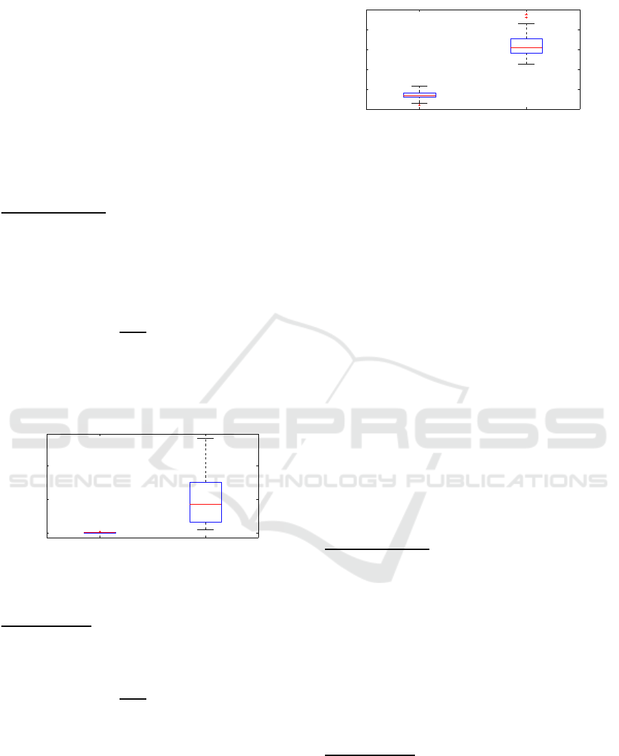
are represented by box plots in Figure 7 for both pop-
ulations. As expected, the global temporal errors of
novices are larger than of experts.
experts novices
0
50
100
Figure 7: Temporal error distribution for novices and the
experts that are not included in the reference database.
Spatial Analysis
To quantify the spatial errors, we applied the same
evaluation process. For each example, we computed
the global spatial errors from local spatial errors:
ERR
spa
=
1
M
L
A
M
L
−1
∑
t=0
A
∑
a=1
E
a
spa
(t)
As shown in Figure 8, box plots of global spatial
errors for the two populations are clearly separated,
experts are distinguished from novices. Moreover er-
rors are larger and more dispersed for novices than ex-
perts, highlighting the worst performance of novices
and the higher variability of their motions.
Our approach can thus easily distinguish novices
from expert players both with spatial and temporal er-
rors.
experts novices
2
3
4
5
Figure 8: Spatial error distribution for novices and the ex-
perts that are not included in the reference database.
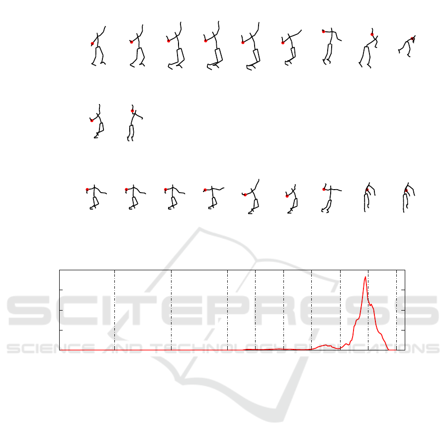
4.2 Evaluation of a Novice’s Motion
The goal of this second experiment is to apply our
method on the motion of a novice player to determine
his/her temporal and spatial errors over time. We
have thus randomly selected one example of novice’s
tennis serve. To better illustrate the results, the
average serve provided by the model of experts
detailed in Section 3.2 is sampled into 9 reference
times {t
1
...t
9
}. The first row of Figure 9 shows the
postures of this average motion at all these times
(with a finer sampling at the end of the motion to have
more details on this most dynamic part). The novice’s
serve is shown on the second row of Figure 9. Since
this novice player made his serve faster, only two
postures are illustrated but of course all the postures
of the motions are considered for the following
analyses. Finally, the third row illustrates how the
novice’s serve was globally aligned by Algorithm 1.
The two motions are temporally coherent and the
errors between them can be evaluated.
Temporal Analysis
To qualitatively analyze the temporal results obtained
on the novice’s motion, the temporal error of the
novice’s right elbow is drawn in Figure 10. The
temporal error is very low for all times except for t
8
where E
a
temp
(t
8
) = 50.48. At this time, the expert is
hitting the ball while the novice is already ending his
motion. This shows that the novice player moved
his arm earlier than the expert relatively to his global
movement. This relative temporal delay between
the motions is obtained thanks to the global optimal
alignment made by Algorithm 1.
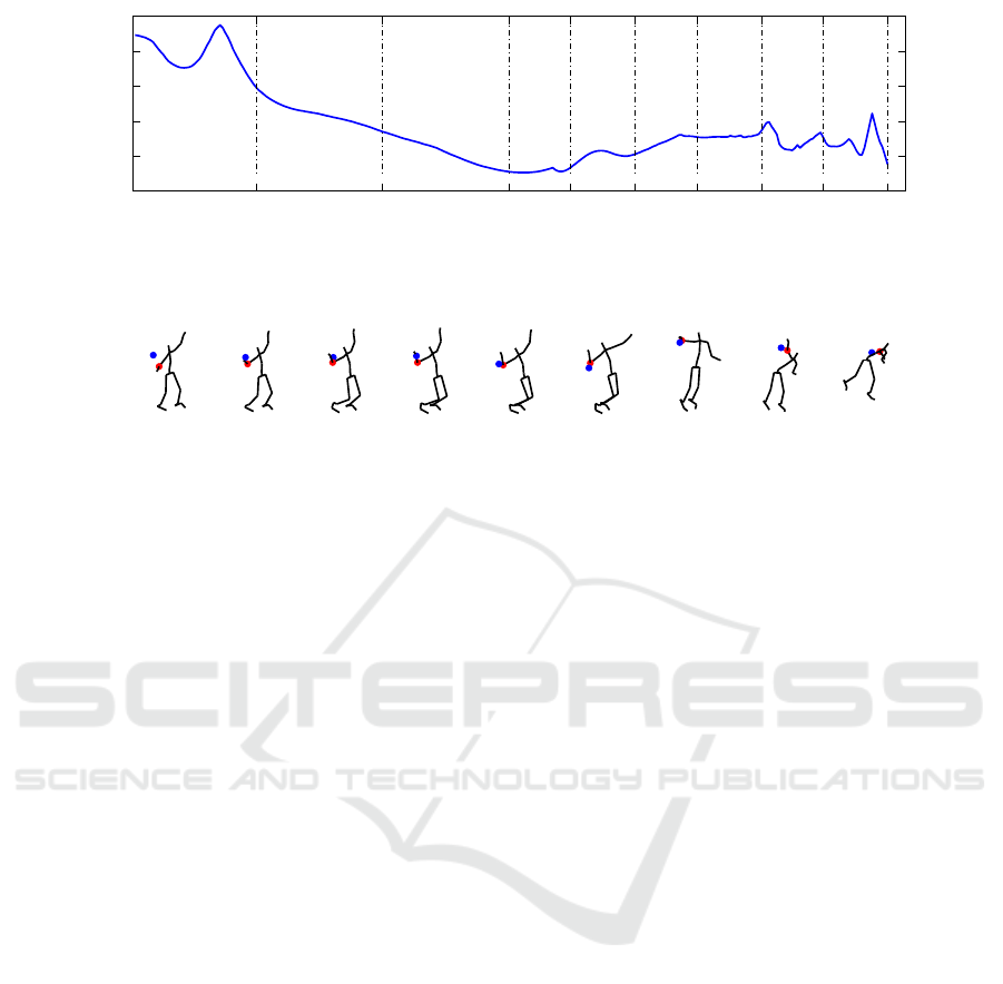
Spatial Analysis
The spatial error computed by our method for the
novice’s right elbow is drawn in Figure 11. The
greater spatial error is obtained at the beginning of the
motion. Figure 12 shows the position of the right el-
bow of the novice (in blue) and of the expert (in red)
above the posture of the average motion of experts.
The main error is indeed located at the beginning of
VISAPP 2016 - International Conference on Computer Vision Theory and Applications
550

t
1
t
2
t
3
t
4
t
5
t
6
t
7
t
8
t
9
Globally
aligned
novice serve
Novice serve
Average
expert serve
Figure 9: First row: average motion provided by our model of experts’ motion, sampled into 9 times for illustration purpose.
Second row: original novice’s motion at the same times. Third row: novice’s serve after alignment with the path P
S
mean
of
Algorithm 1. Red dots correspond to the right elbow of the player.
t1 t2 t3 t4 t5 t6 t7 t8 t9
0
20
40
60
80
Temporal error
Figure 10: Temporal error of the novice’s right elbow over time. The 9 reference times illustrated in Figure 9 are represented
by vertical dashed lines.
the motion and is due to a bad technique of the novice:
he did not lowerenough the racket to exploit at best its
displacement to have an optimal speed at ball impact.
Even if these results are preliminary, they high-
light the strength of our method that can take both
spatial and temporal errors into account to accurately
identify the errors over time. Moreover, these errors
are not only global information but are precise enough
to point out local errors such as the synchronization
between limbs or the spatial and temporal error of a
joint relatively to the global motion. All these out-
comes are moreover obtained independently of the
length of the motions.
5 CONCLUSION
In this paper, we proposed an innovative approach to
automatically evaluate sport motions independently
to the type of sport or the morphology of the player.
Preliminary results showed that our algorithm can
correctly distinguish novice players from experts but
even better it can quantify over time the temporal and
spatial errors of the performance of a novice player
compared to a database of experts. These results were
achieved thanks to a 2-level DTW. Actually, a single
DTW can only give information about the global er-
ror of the motion without considering the temporality
between limbs for instance and without localizing the
errors. Another solution could have been to manage
each joint independently but no relationships between
the joints could then be identified. Our solution over-
comes these limits: both spatial and temporal features
are considered concurrently and can then be used to
propose an accurate training solution to work on that
specific imperfections of the gesture and at the right
time.
Our algorithm is based on a random-based selec-
tion process that could make it stochastic and then
subject to variations. On the contrary, this process al-
Automatic and Generic Evaluation of Spatial and Temporal Errors in Sport Motions
551

t1 t2 t3 t4 t5 t6 t7 t8 t9
0
2
4
6
8
10
Spatial error
Figure 11: Spatial error of the novice’s right elbow over time. The 9 reference times illustrated in Figure 9 are represented by
vertical dashed lines.
t
1
t
2
t
3
t
4
t
5
t
6
t
7
t
8
t
9
Figure 12: Position of the right elbow of the experts’ average motion (red) and of the novice’s one (blue) after local alignment
P
RElb
mean
.
lows the detection of outliers, i.e. joints that are badly
synchronized with others, in an efficient way. How-
ever, these preliminary results must be extended to a
bigger population to have a statistical analysis.
This approach opens wide range of use cases.
It can indeed be used to automatically compare
the novice’s motion of any individual sport to the
database of expert without adding knowledge or edit-
ing/annotating the experts’ motions. But it can also be
used to compare a novice or injured player along time
to evaluate his/her progression. This method could
thus be the core of a generic and automatic training
system to be used complementary to traditional train-
ing sessions.
ACKNOWLEDGEMENTS
The data used in this project was obtained from a ten-
nis project carried out in the M2S laboratory. The
authors thank Caroline Martin and Pierre Touzard for
this supply.
REFERENCES
Barnachon, M., Bouakaz, S., Boufama, B., and Guillou,
E. (2013). A Real-Time System for Motion Re-
trieval and Interpretation. Pattern Recognition Letters,
34(15):1789–1798.
Burns, A.-M., Kulpa, R., Durny, A., Spanlang, B., Slater,
M., and Multon, F. (2011). Using virtual humans and
computer animations to learn complex motor skills: a
case study in karate. BIO Web of Conferences, 1(12).
Gong, D., Medioni, G., and Zhao, X. (2014). Structured
time series analysis for human action segmentation
and recognition. IEEE Transactions on Pattern Anal-
ysis and Machine Intelligence, 36(7):1414–1427.
Heloir, A., Courty, N., Gibet, S., and Multon, F. (2006).
Temporal alignment of communicative gesture se-
quences. Computer Animation and Virtual Worlds,
17(3-4):347–357.
Kahol, K., Tripathi, P., and Panchanathan, S. (2004). Com-
putational analysis of mannerism gestures. In ICPR,
pages 946–949.
Keogh, E. J. and Pazzani, M. J. (2001). Derivative dynamic
time warping. In SIAM International Conference on
Data Mining, pages 1–11.
Komura, T., Lam, B., Lau, R. W. H., and Leung, H. (2006).
e-learning martial arts. In ICWL, pages 239–248.
Kulpa, R., Multon, F., and Arnaldi, B. (2005). Morphology-
independent representation of motions for interactive
human-like animation. Computer Graphics Forum,
24(3):343–352.
Maes, P.-J., Amelynck, D., and Leman, M. (2012). Dance-
the-music: an educational platform for the mod-
eling, recognition and audiovisual monitoring of
dance steps using spatiotemporal motion templates.
EURASIP Journal on Advances in Signal Processing,
2012(1):35.
Müller, M. and Röder, T. (2006). Motion templates for au-
tomatic classification and retrieval of motion capture
data. ACM SIGGRAPH, pages 137–146.
Müller, M., Röder, T., and Clausen, M. (2005). Efficient
content-based retrieval of motion capture data. ACM
Transactions on Graphics, 24(3):677.
Ofli, F., Chaudhry, R., Kurillo, G., Vidal, R., and Bajcsy,
R. (2012). Sequence of the most informative joints
(SMIJ): A new representation for human skeletal ac-
tion recognition. In CVPRW, pages 8–13.
Pazhoumand-Dar, H., Lam, C.-P., and Masek, M. (2015).
Joint movement similarities for robust 3D action
VISAPP 2016 - International Conference on Computer Vision Theory and Applications
552

recognition using skeletal data. Journal of Visual
Communication and Image Representation, 30:10–21.
Pham, M. T., Moreau, R., and Boulanger, P. (2010). Three-
dimensional gesture comparison using curvature anal-
ysis of position and orientation. In EMB, pages 6345–
6348.
Röder, T. (2006). Similarity, Retrieval, and Classification
of Motion Capture Data. PhD thesis, Rheinischen
Friedrich- Wilhelms- Universität, Bonn.
Sakoe, H. and Chiba, S. (1978). Dynamic programming
algorithm optimization for spoken word recognition.
IEEE Transactions on Acoustics, Speech, and Signal
Processing, 26(1):43–49.
Sakurai, K., Choi, W., Li, L., and Hachimura, K. (2014).
Retrieval of similar behavior data using kinect data.
In ICCAS, pages 97–104.
Shin, H. J., Lee, J., Shin, S. Y., and Gleicher, M. (2001).
Computer puppetry: An importance-based approach.
ACM Transactions on Graphics, 20(2):67–94.
Sie, M.-S., Cheng, Y.-C., and Chiang, C.-C. (2014). Key
motion spotting in continuous motion sequences using
motion sensing devices. In ICSPCC, pages 326–331.
Sorel, A., Kulpa, R., Badier, E., and Multon, F. (2013).
Dealing with variability when recognizing user’s per-
formance in natural 3D gesture interfaces. Interna-
tional Journal of Pattern Recognition and Artificial
Intelligence, 27(8):19.
Wang, J., Liu, Z. L., Wu, Y. W., and Yuan, J. (2012). Mining
actionlet ensemble for action recognition with depth
cameras. In CVPR, pages 1290–1297.
Wang, S. B., Quattoni, A., Morency, L.-P., and Demirdjian,
D. (2006). Hidden conditional random fields for ges-
ture recognition. In CVPR, pages 1521–1527.
Ward, R. E. (2012). Biomechanical Perspectives on Clas-
sical Ballet Technique and Implications for Teaching
Practice. PhD thesis, University of New South Wales,
Sydney, Australia.
Xia, L., Chen, C.-C., and Aggarwal, J. K. (2012). View
invariant human action recognition using histograms
of 3D joints. In CVPRW, pages 20–27.
Zhong, S. and Ghosh, J. (2002). HMMs and coupled HMMs
for multi-channel EEG classification. In IJCNN, pages
1154–1159.
Zhou, F. and de la Torre, F. (2015). Generalized canonical
time warping. IEEE Transactions on Pattern Analysis
and Machine Intelligence, pages 1–1.
Zhou, F. and De La Torre Frade, F. (2009). Canonical time
warping for alignment of human behavior. In NIPS,
pages 2286–2294.
Automatic and Generic Evaluation of Spatial and Temporal Errors in Sport Motions
553