VOPT: Robust Visual Odometry by Simultaneous Feature Matching and

Camera Calibration

Rafael F. V. Saracchini

, Carlos Catalina

, Rodrigo Minetto

and Jorge Stolﬁ

Dept. of Simulation and Control, Technological Institute of Castilla y Len, Burgos, Spain

Dept. of Informatics, Federal University of Technology, Paran

a, Curitiba, Brazil

Institute of Computing, State University of Campinas, Campinas, Brazil

Keywords:

3D Tracking, Augmented Reality, Camera Calibration, Real-time and GPU Processing.

Abstract:

In this paper we describe VOPT, a robust algorithm for visual odometry. It tracks features of the environ-

ment with known position in space, which can be acquired through monocular or RGBD SLAM mapping

algorithms. The main idea of VOPT is to jointly optimize the matching of feature projections on successive

frames, the camera’s extrinsic matrix, the photometric correction parameters, and the weight of each feature

at the same time, by a multi-scale iterative procedure. VOPT uses GPU acceleration to achieve real-time per-

formance, and includes robust procedures for automatic initialization and recovery, without user intervention.

Our tests show that VOPT outperforms the PTAMM algorithm in challenging videos available publicly.

1 INTRODUCTION

Visual odometry (VO) is the determination of the mo-

tion of a video camera relative to a static environment

by comparing successive video frames (Scaramuzza

and Fraundorfer, 2011). This technique is used in sev-

eral applications in the ﬁeld of robotics, entertainment

and autonomous navigation of terrestrial and aerial

vehicles (Weiss et al., 2013). Speciﬁcally, it is a core

component in most simultaneous tracking and map-

ping (SLAM) algorithms, which acquire a 3D model

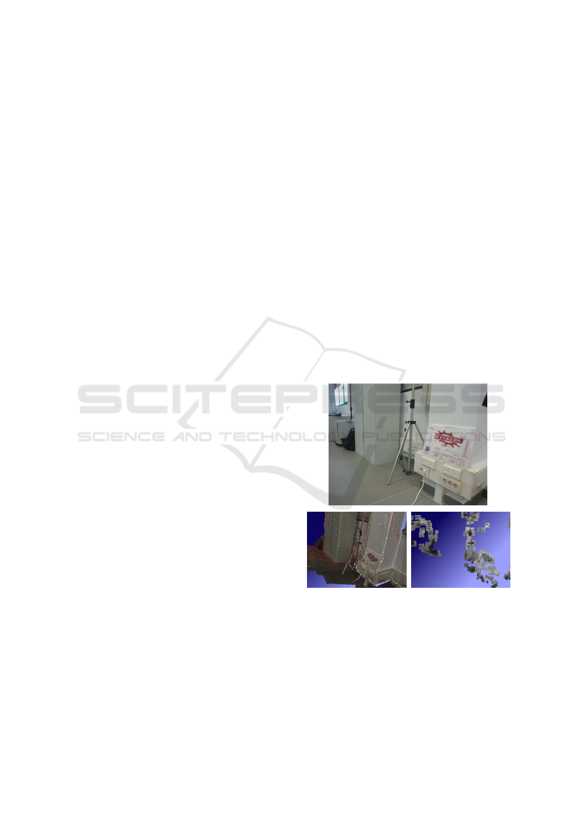
of the environment as it is traversed. See ﬁgure 1.

The contribution of this paper is a robust and ef-

ﬁcient algorithm for visual odometry, which we call

VOPT, with a GPU-based real-time implementation.

The VOPT algorithm uses a sparse model of the en-

vironment, consisting of an unstructured collection

of salient points in 3-space (optionally with surface

normals) that are associated to salient features of the

video frames. The positions and normals of those

tracked features can be obtained either by multiview

stereo or RGBD cameras. Our proposed method also

uses local photometric adjustments of individual fea-

tures to cope with variations in lighting, and is rela-

tively insensitive to motion blur and image noise.

This paper is organized as follows. The environ-

ment model and the algorithm are described in Sec-

tions 2 and 3. We describe our tests in Section 4 and

conclusions in Section 5.

(a) (b)

Figure 1: Input frame and associated visual odometry refer-

ence maps: (a) dense depth map and (b) sparse patch map.

1.1 Related Work

Most VO algorithms can be divided in three classes:

feature-based, appearance-based and patch-based.

Feature-based algorithms (Concha and Civera,

2014; Castle et al., 2008) identiﬁes a large set of dis-

Saracchini, R., Catalina, C., Minetto, R. and Stolﬁ, J.

VOPT: Robust Visual Odometry by Simultaneous Feature Matching and Camera Calibration.

DOI: 10.5220/0005781700590066

In Proceedings of the 11th Joint Conference on Computer Vision, Imaging and Computer Graphics Theory and Applications (VISIGRAPP 2016) - Volume 3: VISAPP, pages 61-68

ISBN: 978-989-758-175-5

tinguished features (such as corners and edges) in a

frame, matching them with a reference set and esti-

mating motion accordingly. By computing the posi-

tions of features with known 3D position its possible

estimate the camera motion position for each captured

frame. The most popular algorithm of this class is

PTAMM (Castle et al., 2008) and its variants (Klein

and Murray, 2009; Weiss et al., 2013). This class

of algorithms is relatively insensitive to lighting vari-

ations and occlusions. However, the feature detection

step is rather costly, since it must allow for afﬁne dis-

tortions of the feature’s image between frames (Lowe,

2004; Bay et al., 2006; Alcantarilla et al., 2013). Such

algorithms are also badly affected by motion blur and

noise.

An appearance-based algorithm requires a 3D ge-

ometric model of the environment, and tries to de-

termine the camera pose for each frame by minimiz-

ing the difference between each observed frame and

a rendering of that model with the tentative camera

position. This approach was used by the DTAM algo-

rithm of Newcombe et al. (Newcombe et al., 2011b)

algorithm, which used a dense depth map representa-

tion. In order to reduce computational costs, Engel et

al. (Engel et al., 2013) and Forster et al. (Forster et al.,

2014) proposed the use of a semi-dense model con-

taining only the parts of the depth map near salient

elements like edges and corners. These methods are

less sensitive to motion blur and noise but are sensi-

tive to lighting variations (although lighting variations

can be alleviated by using dense maps (Maxime et al.,

2011)).

A patch-based algorithm follows an intermediate

approach. It uses a very sparse model of the envi-

ronment, consisting of a set of ﬂat patches of the en-

vironment’s surface, with known 3D positions, ap-

pearance, and normal vectors. For each frame, the

camera position is adjusted until the computed projec-

tions of these surface patches match the correspond-

ing parts of the frame image. Examples of this class

are the Vachetti et al. (Vacchetti et al., 2004), and

the AFFTRACK algorithm of Minetto et al. (Minetto

et al., 2009). These algorithms have lower computa-

tional cost than appearance-based algorithms because

they don’t have to do a full rendering of the environ-

ment model for each tentative camera pose; and also

lower cost than feature-based algorithms because they

can predict the position and deformation of each patch

caused by the camera motion. VOPT can use ei-

ther the feature-based approach or the patch-based ap-

proach, depending on the availability of surface data.

2 DATA REPRESENTATION

Video Frames. A video is assumed to be a sequence

of N images F

,...,F

N−1

, the frames, all with n

columns by n

rows of pixels. Each frame F

can be

viewed as a function from the rectangle D = [0,n

] ×

[0,n

] of R

to some color space, that is derived from

the pixel values by some interpolation schema.

Camera Model. We denote by ρ the projection func-

tion that maps a 3D point p of C to a 2D point q of

D belong to a frame, where C ⊂ R

is the cone of

visibility of the camera. We assume a pinhole cam-

era model, so that the projection is determined by the

3 × 4 homogeneous intrinsic matrix K of the camera

that deﬁnes the projection from the camera’s coor-

dinate system to the image sensor plane, and by the

4×4 homogeneous extrinsic matrix T that deﬁnes the

current position and pose of the camera relative to the

world’s coordinate system. We assume K known and

radial distortion removed a priori and that the camera

has ﬁxed focal length (zoom), so that the K matrix is

the same for all video frames. We also assume that

the video frames have been corrected and do not have

any radial distortions.

The projection function ρ is deﬁned by

q = ρ

K,T

(p) = KT

−1

p (1)

where p and q are represented as homogeneous co-

ordinate column vectors. Note that the T matrix in-

cludes the 3 coordinates of the camera’s position and

a 3 × 3 orthonormal rotation submatrix. We denote

by ~v(T, p) the unit direction vector in space from the

point p ∈ R

to the position of the camera implied

by the extrinsic matrix T and the projection function

K,T

(p) which maps a point p ∈ R

into image coor-

dinates.

Tracked Features. The essential information about

the environment is a list S = (s

,...,s

n−1

) of fea-

tures on its surface. Each feature s

has a space po-

sition s

.p in R

and (optionally) a local surface nor-

mal s

.~u ∈ S

. (By convention, s

.~u is (0, 0, 0) if the

normal is not available.) Each feature s

is also asso-

ciated to a sub-image of some reference image s

.J ,

called the canonical projection of the feature. We will

assume that all reference images have the same do-

main D

∗

= [0, n

∗

] × [0,n

∗

] and were imaged with the

same intrinsic camera matrix K

∗

. The canonical pro-

jection of the feature is represented in the algorithm

by a pointer to the reference image s

.J , the extrinsic

camera matrix s

.T already determined for that refer-

ence image, a bounding rectangle s

.R ⊂ D

∗

, and a

mask s

.M . The mask is a pixel array with values in

[0,1], spanning that rectangle, that deﬁnes the actual

VISAPP 2016 - International Conference on Computer Vision Theory and Applications

Figure 2: Projection of features s

and s

on the image K =

.J = s

.J , showing their bounding rectangles s

.R,s

(left) and their masks s

.M ,s

.M (right).

extend and shape of the image feature on the reference

image. See ﬁgure 2.

Key Frames an Pose Graph. In order to start the

tracking, and restart it after a tracking failure, the al-

gorithm requires a list K = (K

∗

,...,K

∗

−1

) of

reference images of the environment, the key frames.

Speciﬁcally, for each key frame K

∗

∈ K , the algo-

rithm requires an extrinsic matrix T

∗

and a set S

∗

features that are visible in it. It also requires a pose

graph G, whose vertices are the key frames, with an

edge between two key frames if their views have suf-

ﬁcient overlap.

This Key Frame Data can be obtained from several

sources: frame squences, depth maps from with de-

vices like laser rangers and RGBD cameras, structure-

from-motion, etc. The feature set and pose graph are

then derived from sparse (Castle et al., 2008; En-

gel et al., 2013) or dense (Newcombe et al., 2011a;

Whelan et al., 2012) maps computed by SLAM algo-

rithms. The masks s

.M can be determined by back-

projecting the bounding rectangle s

.R into the scene

geometry, discarding regions which are not connected

to its centre and computing a weight proportional with

the difference of the surface normal with s

.~u. In case

of sparse maps, the mask is not computed and all its

values are set to 1.

3 TRACKING ALGORITHM

The VOPT algorithm is applied to each frame I = F

of a video sequence. Its normal case is described in

ﬁgure 3. It takes as inputs the collection of tracked

space features S, and the previous video frame I

i−1

with its extrinsic camera matrix T

. For each

feature s

in S it also receives the reliability weight

that measures its visibility in frame I

and how

well it matched its canonical projection. If success-

ful, the procedure returns the extrinsic matrix T for

frame I , and, for each feature s

, an adjusted weight

. It requires an startup procedure (Straub et al.,

Procedure VOPT(S,I , I

) returns (T,w)

1. (d,w) ← DISPLACEMENTS(S,I

,I )

2. (T,w) ← ESTIMCAMERA(S, T

,d,w);

3. (T,w) ← CAMADJUST(S, I , T,w)

Figure 3: The normal case of the VOPT algorithm.

2013; Saracchini and Ortega, 2014) to select the fea-

tures S to be tracked on the ﬁrst image of the video,

I = F

, the extrinsic matrix T

. We used the approach

described in (Saracchini and Ortega, 2014) in order

to initialize the system and select the most likely key-

frames and associated features from the pose-graph

map. This procedure will be brieﬂy described in sec-

tion 3.3.

The VOPT algorithm can be summarized as fol-

lows:

The procedure DISPLACEMENTS in step 1 ﬁrst com-

putes the position c

of each feature pont s

.p with

> 0 on frame I

, using the corresponding camera

matrix T

. Then it uses the multiscale KLT algorithm

of Kanade et al. (Shi and Tomasi, 1994) to determine

the optical ﬂow Φ : D → D between the frames I

and

I . For efﬁciency, the ﬂow is computed only in a sub-

set of the domain, consisting of the union of 21 × 21

pixel squares centred at the points c

. The ﬂow Φ is

applied to the center c

= ρ

K,T

.p) of each feature

projection in I

to obtain its approximate apparent po-

sition c

in I . Note that each feature is independently

mapped, without considering the constraints of per-

spective change. The procedure returns the displace-

ment d

= c

− c

∈ R

between the projected feature

positions on frame I

and their apparent positions on

frame I . The weight w

of each feature is set to zero

if w

= 0, or if any of these steps fails (e.g. if c

falls

outside D).

In step 2, an initial estimate of the camera matrix

T is obtained from the 3D position s

.p of each fea-

ture, the camera matrix T

of the previous frame, and

its apparent displacement d

between the two frames.

We use Klein’s iterative M-Estimator (Klein, 2006),

except that the diagonal weight matrix W is computed

by the formula

2k,2k

= W

2k+1,2k+1

= w



1 +



−1

(2)

where r

the residual of the computed and observed

displacement is the Euclidean length of the difference

between the observed displacement d

and the dis-

placement computed from the 3D position s

.p, the

matrix T

, and the current version of the matrix T .

The M-estimator algorithm usually converges in 10

to 20 iterations. At the end, each reliability weight

is updated from the weight matrix W , by inverting

formula (2).

VOPT: Robust Visual Odometry by Simultaneous Feature Matching and Camera Calibration

In step 3, the initial estimate of the extrinsic matrix

T for frame I (wich is often imprecise, due to errors

in the displacements d

) is iteratively reﬁned by the

procedure CAMADJUST, simultaneously with the re-

liability weight w

for each tracked feature s

. This

step is detailed in section 3.1.

3.1 Camera Pose Reﬁnement

The procedure CAMADJUST receives as input the

list S of features that are being tracked, their cur-

rent weights w

, the next frame I , and an initial es-

timate T of its extrinsic matrix. It returns the ad-

justed matrix T and an updated reliability weight w

for each feature. The procedure is similar to the core

of the AFFTRACK (Minetto et al., 2009). It adjusts

the camera matrix T and the reliability weights w

it-

eratively for each level l of a image pyramid, by re-

ﬁning the apparent positions the features on the cur-

rent frame, allowing for differences in illumination

between the canonical projection and the current pro-

jection of each feature. Features that are not visible

eventually get w

set to zero, and excluded from the

computation of T . See ﬁgure 4.

Procedure CAMADJUST(S, I ,T,w) returns (T,w)

1. Repeat while T does not converge, or until N

iterations:

2. For each feature s

in S,

3. Let P

← GETLOCALMAP(s

,T )

4. d

← (0, 0)

5. For each level ` from N

− 1 down to 0, do

6. For each feature s

with a valid map P

7. Scale P

to level `.

8. (d

) ←

FADJUST(s

(`)

)

9. (T,w) ← ESTIMCAMERA(s, T, d,w)

Figure 4: The iterative camera adjustment procedure.

Each iteration of CAMADJUST ﬁrst computes a local

2D projective transformation P

that describes the es-

timated position and deformation of each feature s

from its key frame s

.J to the image I , due to cam-

era motion between the two frames, assuming the cur-

rent guess for the matrix T. Then, for each feature s

the procedure determines a displacement d

from that

estimated position to the position that yields the best

match with the contents of frame I .This displacement

is computed by incremental adjustments at multiple

scales of resolution. Finally, the displacements d

are

used to correct the matrix T , by Klein’s M-Estimator.

The iteration stops when the adjusted matrix T does

not change signiﬁcantly, or after N

iterations.

Feature Deformation Map. The projective map P

computed in step 3 is obtained by lifting the rectangle

.R to 3D space and projecting it onto the frame I .

More precisely, let Π

be a plane in R

that passes

through the point s

.p and is perpendicular to the

surface normal s

.~u. If the surface normal s

.~u is

not known, then Π is assumed to be perpendicular

to ~v(S,s

.p). Each corner p of the rectangle s

.R is

mapped to a point q of R

q = ρ

K,T

(ρ

−1

∗

,S,Π

(p)) (3)

where S = s

.T is the extrinsic matrix of the key frame

of that feature, and ρ

−1

∗

,S,Π

is the function that back-

projects that key frame onto the plane Π

. However,if

.~u ·~v(T, s

.p) ≤ 0, or if a corner lies outside D, the

feature is considered invisible (self-occluded) in the

frame I . and the map P

is not deﬁned. If the pro-

jected corners fall behind the camera or outside D the

feature is considered invisible, and P

invalid.

Multiscale Processing. In order to achieve robust

and efﬁcient discovery of large (multi-pixel) displace-

ments, the feature adjustment step 8 is repeated at

multiple scales of resolution, using an image pyramid

(0)

= I , I

(1)

, I

−1)

, each level I

(`)

being scaled

by 1/2

in each axis. Note that the weights w

are

recomputed from scratch at each level.

Note also that the map P

and the accumulated dis-

placement d

are initially scaled by 1/2

−1

and then

scaled by 2 when going from one level to the next

ﬁner level. At each level, the FADJUST procedure can

only adjust the displacement d

by a few pixels. How-

ever, because of the multiscale processing, the total

displacement can be of the order of 2

−1

pixels on

the original images.

3.2 Image Feature Position Adjustment

The FADJUST procedure is called for each feature s

and scale l, to reﬁne the position of the feature on

the frame I . The procedure receives a 2D projective

map that deﬁnes the position and shape of the feature

on I , computed from the current guess of the matrix

T for that frame; and a displacement d

found by

image matching at coarser scales. First, the procedure

estimates the changes in the lighting of the feature

between those two frames, then it applies a small

correction to the displacement d

with the Lucas-

Kanade local image matching algorithm (Birchﬁeld,

2014). The weight w

of each feature is deﬁned based

on the quality of the match. See ﬁgure 5.

Photometric Correction. The procedure

PHOTOCORR in step 3 determines the correc-

tion of pixel values under lighting effects, which is

needed to compensate for changes in illumination

VISAPP 2016 - International Conference on Computer Vision Theory and Applications

Procedure FADJUST(s

,I ,d

) returns (d

)

1. Set R

to the bounding box of P

.R) dis-

placed by d

2. If R

is contained in D and has at least 4 rows

and 4 columns,

3. (α

,β

) ← PHOTOCORR(s

,I )

4. If α

≥ α

min

5. (d

) ← LK(s

,I ,α

,β

)

6. else set w

← 0

7. else set w

← 0

Figure 5: The local feature position adjustment procedure.

between the two frames, including the effects of shad-

owing, surface orientation, glossy highlights, etc. We

assume that these effects can be well approximated

by an afﬁne function I (P

(p) + d

) ≈ α

K (p) + β

for any point p within the mask N = s

.M ; where

K = s

.J . Basically, α

is the relative change in

contrast, and β

captures the difference of the ‘black

levels’ of the two images around the respective

projections of the feature. The values of α

and β

are obtained by weighted least squares, using the

squared discrepancy Q deﬁned by

Q(d

,α

,β

) =

∑

p∈s

N (p)(α

K (p)+β

−I (P

(p)+d

))

(4)

for the given value of the displacement d

. If α

negative (meaning that darker areas of the canonical

projection became lighter on the current image, and

vice-versa) or zero, the procedure consider the feature

lost and/or obscured by pixel noise, setting the weight

to zero. On the other hand, β

can be positive or

negative.

Local Feature Matching. In step 5, the Lucas-

Kanade (LK) algorithm (Birchﬁeld, 2014) is used to

adjust the displacement d

so that the pixel values of

I are most similar to those of K = s

.J , after mapped

by P

, displaced by d

, and color-corrected accord-

ing to α

and β

. The similarity is evaluated by the

same Q functional (4) used for photometric correc-

tion. If the LK algorithm does not converge after N

iterations, we consider the adjustment failed, and set-

ting w

to zero. Otherwise we set w

to exp(−z

/2),

where z = Q/(α

) and σ is the expected standard

deviation of the pixel noise.

GPU Acceleration. Steps 3 and 5 of FADJUST are

responsible for most of the computational cost of

the VOPT algorithm, requiring computation of sums

over all pixels of a feature projection, mapped by the

deformation map P

. We compute those sums on GPU

by parallel reduction (Harris et al., 2007; Micikevi-

cius, 2009), and warping images by bi-cubic inter-

polation (Ruijters et al., 2008) using texture memory,

which is initialized in the startup procedure. The key

frames s

.J and the image feature masks s

.M are

copied into the GPU’s texture memory, and the tex-

ture warping functions are used to map the pixel po-

sitions in the key frame to the current frame by fast

cubic interpolation (Ruijters et al., 2008). Those two

steps require solving 2 × 2 linear systems, which are

solved in the CPU.

3.3 Initialization and Recovery

The VOPT algorithm requires an auxiliary startup

procedure to select the features to be tracked on the

ﬁrst image of the video, I = F

, and to deﬁne the

extrinsic matrix T

for that frame. This procedure is

also needed to restart the odometry if the VOPT al-

gorithm fails, e.g. because there are not enough fea-

tures that are visible in the frame (speciﬁcally, if the

CAMADJUST procedure ends with fewer than 5 fea-

tures with non-zero weight w

). If VOPT fails when

trying to go from some frame I

= F

i−1

to the next

frame I = F

, we give up on that frame and apply the

startup procedure to frame I = F

i+1

The startup procedure looks for the most similar

key-frame K

∗

in K to the target image I by feature-

matching, using the vocabulary tree technique of Nis-

ter and Stewenius (Nister and Stewenius, 2006) and

extended in (Saracchini and Ortega, 2014). After-

wards, we build a list S of features to be tracked as

the union of S

∗

and of all S

∗

such that K

∗

is adja-

cent to K

∗

in the pose graph G. The startup pro-

cedure then computes an approximate estimate T for

the matrix of frame I using RANSAC. Finally it uses

the CAMADJUST procedure to improve the estimated

camera pose. This procedure, although very robust,

is noticeably slower than the odometry procedure due

the high computational cost of detecting and match-

ing features.

4 EXPERIMENTS

Test Videos. We tested the VOPT algorithm on both

synthetic and real video sequences. See Table 1. In

all tests, we set N

= 2, N

= 10 iterations, N

= 3

pyramid levels, α

min

= 0, and σ = 0.1. All the al-

gorithms were tested in standard PC with an Intel i5

3.2 Ghz, 4GB of RAM, and Geforce 650 GTX graph-

ics card. The operational system was Linux Debian

”wheezy” 64-bit.

The real videos were captured with a hand-held

Logitech C930 camera, recording 840 × 480 frames

at 30 fps, with ﬁxed focal length. The intrinsic cam-

era matrix K was determined by OpenCV calibration.

One set of real videos (group M) was obtained by mov-

ing the C930 camera back and forth over a cluttered

VOPT: Robust Visual Odometry by Simultaneous Feature Matching and Camera Calibration

Table 1: Video dataset information. Notes: videos with (o)

feature occlusion, (m) motion, (l) adverse lighting, (b) mo-

tion blur and (*) navigation in unmapped regions.

Video Frames Notes

S0 241 [m]

S1 241 [o,m]

Synthetic

S2 241 [b,m]

S3 241 [o,b,m]

S4 241 [l,m]

S5 241 [l,o,m]

S6 241 [l,b,m]

S7 241 [l,b,o,m]

Real

M0 711 [o,m]

M1 510 [o,b,m]

C0 1207 [o,b,m]

C1 425 [o,b,m]

C2 1015 [o]

C3 709 [o,m]

C4 666 *[o,b,m]

ofﬁce desk. Another set of videos (group C) was taken

by walking down a laboratory corridor with the cam-

era.

The synthetic videos (group S) were generated by

rendering a 3D model of an abbey with the Blender

ray-tracer (Blender Online Community, 2014).For

each video frame F

, we saved the corresponding ex-

trinsic camera matrix T

used in the rendering. We se-

lectively enabled challenging factors such as motion

blur, localized illumination by spotlights, and occlu-

sion by several objects.

Key Frame Data. For each of the groups S, M, and

C, we used the PTAMM (Castle et al., 2008) to obtain

one set KPT of key frame data, including the set of key

frames K , the pose graph G, and, for each key frame

∗

, the extrinsic matrix T

∗

, and the set of features S

∗

using a reference video without adverse effects. The

input to PTAMM was a reference video in plain RGB

format, distinct from the test videos. For the M and

C groups, the reference video was acquired with the

C930 camera. For the S group, the reference video

was rendered with Blender, without the extra chal-

lenging factors. For each key-frame, we discarded

redundant features, accepting at most 60, and a total

limit of 180.

We also tested the algorithm with reference maps

obtained from depth 3D reconstruction. For the the

groups S and C, we produced a set KSO of key frames

containing dense data, constructing the pose-graph

map with a RGBD-SLAM algorithm (Saracchini and

Ortega, 2014) for the C group and by depth-map ren-

dering the 3D model of the abbey at regularly spaced

intervals for the S group. The feature sets S

∗

were

extracted by using a corner detector (Shi and Tomasi,

1994), discarding regions without depth, and normals

computed directly from the depth map.

Algorithms and Metrics. For each test video, we

ran the VOPT algorithm with the KPT key frame

data set (S, M, and C groups) and with the KSO data

set (S and C groups). For comparison, we also ran

the visual odometry module of PTAMM (PTAMM-

VO) on each video with its original frame data with

the key frame data KPT obtained by PTAMM, ex-

cept that the feature sets were not trimmed. For

each test run, we recorded the fraction κ of frames

that were successfully calibrated (either by the startup

procedure or by VOPT), the number L of tracking

losses and average processing time per frame t in mil-

liseconds. For the synthetic videos, we also com-

puted the RMS error ¯e between the estimated T

and

the ground-truth T

. The test videos, key frame

data sets, and outputs of all these runs are available

at http://www.liv.ic.unicamp.br/ saracchini/VOPT/.

Results. Our results are summarized in ﬁgures 6, 7

and Table 2. It can be seen that VOPT was gener-

ally more accurate (smaller ¯e) and robust (larger κ,

smaller L), outperforming PTAMM using less data

and achieving best results when using dense data

KSO and in both cases it performed much better than

PTAMM-VO. The latter failed more often, and had

more difﬁculty in recovery, in the presence of light-

ing variations, motion blur, and occlusions. It failed

only with extreme motion blur or in absence of vis-

ible features, which is the case of video C4. VOPT

executed in 9–45 ms, depending on the number of it-

erations needed in steps 2–1 of CAMADJUST and of

the Lucas-Kanade step 5 in FADJUST. Recovery after

failure was much slower (50− −180 ms) due the high

cost of feature matching. In comparison, PTAMM

processed each frame in 8 − −10 ms.

5 CONCLUSIONS

Our tests show that the VOPT algorithm is slight

slower than PTAMM’s visual odometry mode, but is

considerably more accurate and robust, especially in

the presence of motion blur, occlusions, and localized

lighting variations. It owes these qualities mainly to

the simultaneous adjustment of the camera matrix, the

photometric correction parameters, and the reliability

weights of individual features. VOPT was also used

with success in indoor navigation algorithms of an as-

sisted living device with on-site AR capabilities (NA-

CODEAL, 2014).

Besides its robustness, the proposed algorithm

still have limitations which shall be overcome in fu-

ture works. Namely, it depends on an associated

SLAM method to compute the features data needed

VISAPP 2016 - International Conference on Computer Vision Theory and Applications

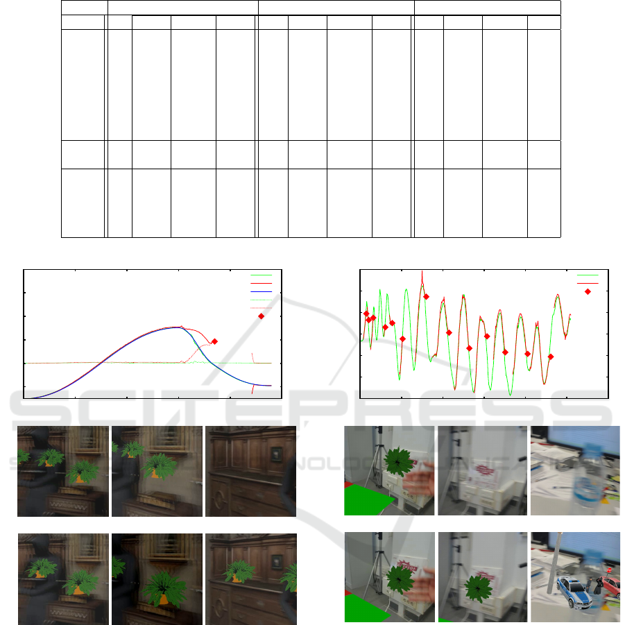
Table 2: Tests with computed values of L (tracking losses), κ (successfully calibration), ¯e (RMS error) and t (time in ms).

Video VOPT (sparse - KPT) VOPT (dense - KSO) PTAMM-VO

L κ ¯e t L κ ¯e t L κ ¯e t

S0 0 1.00 0.048 16.9 0 1.00 0.008 18.8 0 0.98 0.042 3.4

S1 0 1.00 0.049 18.6 0 1.00 0.008 20.9 0 0.98 0.043 3.2

S2 0 1.00 0.062 17.2 0 1.00 0.055 19.5 1 0.85 1.002 2.9

S3 0 1.00 0.061 19.2 0 1.00 0.082 21.6 1 0.84 0.732 2.8

S4 0 1.00 0.042 18.9 0 1.00 0.009 22.1 3 0.79 7.679 1.9

S5 0 1.00 0.037 19.6 0 1.00 0.012 23.1 3 0.48 2.897 3.0

S6 0 1.00 0.060 20.2 0 1.00 0.046 25.1 2 0.11 1.507 1.2

S7 0 1.00 0.064 20.7 0 1.00 0.051 24.8 2 0.14 4.774 1.1

M0 0 1.00 - 27.3 - - - - 6 0.92 - 2.1

M1 0 1.00 - 30.7 - - - - 13 0.67 - 3.1

C0 2 0.99 - 15.2 0 1.00 - 15.5 10 0.52 - 1.8

C1 1 0.97 - 14.9 0 1.00 - 18.8 2 0.88 - 2.0

C2 0 1.00 - 12.3 0 1.00 - 14.6 4 0.79 - 2.1

C3 0 1.00 - 13.5 0 1.00 - 16.4 3 0.81 - 1.7

C4 9 0.83 - 12.8 11 0.87 - 18.7 11 0.71 - 2.3

-2

0 50 100 150 200 250

frame

VOPT Traj. x

PTAMM Traj. x

Ground-truth Traj. x

VOPT Error. x

PTAMM Error. x

PTAMM L

185

PTAMM

VOPT

(a) S3-165 (b) S3-173 (c) S3-185

Figure 6: Plot of x camera position of sequence S3, and

AR output in the virtual scene with its respective sequence

and frames. Note the increasing drift in the AR output of

PTAMM.

for odometry. It also do not provide an efﬁcient

method to update the list of tracked features from the

map after initialization. In the current implementation

it allows to local tracking only, if the camera moves

outside the region covered by the selected patches a

tracking loss and subsequent reinitialization will fol-

low. Finally the dependency on a GPU makes it less

suitable for devices without a dedicated graphics card.

-1.6

-1.4

-1.2

-1

-0.8

-0.6

-0.4

0 100 200 300 400 500 600

frame

VOPT Traj. x

PTAMM Traj. x

PTAMM L

103

160

215

264

307

351

405

461

PTAMM

VOPT

(a) C0-794 (b) C3-287 (c) M1-354

Figure 7: Plot of x camera position of sequence M1, and

AR output (plant/car) in occurrence of occlusions(a), mo-

tion blur(b) and both conditions(c) with its respective se-

quence and frames.

Future works will involve the development of

light-weight version of VOPT aimed to mobile de-

vices, as well the incorporation of the VOPT as effec-

tive module of a full SLAM system, overcoming the

aforementioned limitations. We aim also for a more

efﬁcient usage of the GPU capabilities by exploiting

cache and spatial locality.

VOPT: Robust Visual Odometry by Simultaneous Feature Matching and Camera Calibration

ACKNOWLEDGEMENTS

This work was funded by the Ambient Assisted Liv-

ing Joint Programme as part of the project Natu-

ral Communication Device for Assisted Living, ref.

AAL-2010-3-116 (NACODEAL, 2014).

REFERENCES

Alcantarilla, P. F., Nuevo, J., and Bartoli, A. (2013). Fast

explicit diffusion for accelerated features in nonlin-

ear scale spaces. In British Machine Vision Conf.

(BMVC).

Bay, H., Tuytelaars, T., and Van Gool, L. (2006). Surf:

Speeded up robust features. In Leonardis, A., Bischof,

H., and Pinz, A., editors, Computer Vision – ECCV

2006, volume 3951 of Lecture Notes in Computer Sci-

ence, pages 404–417. Springer Berlin / Heidelberg.

Birchﬁeld, S. (2014). Derivation of

kanade-lucas-tomasi tracking equation.

https://www.ces.clemson.edu/ stb/klt/birchﬁeld-

klt-derivation.pdf.

Blender Online Community (2014). Blender - a 3D mod-

elling and rendering package. Amsterdam.

Castle, R., Klein, G., and Murray, D. (2008). Video-Rate

Localization in Multiple Maps for Wearable Aug-

mented Reality. In IEEE International Symposium on

Wearable Computers (ISWC), pages 15–22.

Concha, A. and Civera, J. (2014). Using Superpixels in

Monocular SLAM. In IEEE International Conference

on Robotics and Automation (ICRA), pages 365–372.

Engel, J., Sturm, J., and Cremers, D. (2013). Semi-dense

visual odometry for a monocular camera. In IEEE In-

ternational Conference on Computer Vision (ICCV),

pages 1449–1456.

Forster, C., Pizzoli, M., and Scaramuzza, D. (2014). SVO:

Fast Semi-Direct Monocular Visual Odometry. In

IEEE International Conference on Robotics and Au-

tomation (ICRA), pages 15–22.

Harris, M. et al. (2007). Optimizing Parallel Reduction in

CUDA. NVIDIA Developer Technology, 2(4).

Klein, G. (2006). Visual Tracking for Augmented Reality.

PhD thesis, University of Cambridge.

Klein, G. and Murray, D. (2009). Parallel tracking and map-

ping on a camera phone. In IEEE International Sym-

posium on Mixed and Augmented Reality (ISMAR),

pages 83–86.

Lowe, D. G. (2004). Distinctive image features from scale-

invariant keypoints. Int. J. Comput. Vision, 60(2):91–

110.

Maxime, M., Comport, A., and Rives, P. (2011). Real-Time

Dense Visual Tracking under Large Lighting Varia-

tions. In British Machine Vision Conference (BMVC),

pages 45.1–45.11. BMVA Press.

Micikevicius, P. (2009). 3D Finite Difference Computation

on GPUs using CUDA. In Workshop on General Pur-

pose Processing on Graphics Processing Units, pages

79–84. ACM.

Minetto, R., Leite, N., and Stolﬁ, J. (2009). AFFTrack: Ro-

bust Tracking of Features in Variable-Zoom Videos.

In IEEE International Conference on Image Process-

ing (ICIP), pages 4285–4288.

NACODEAL (2014). NACODEAL - Natural Communi-

cation Device for Assisted Living. European Union

Project. www.nacodeal.eu. Ambient Assisted Living

Joint Programme ref. AAL-2010-3-116.

Newcombe, R., Izadi, S., Hillige, O., Molyneaux, D., Kim,

D., Davison, A., Kohli, P., Shotton, J., Hodges, S.,

and Fitzgibbon, A. (2011a). KinectFusion: Real-time

Dense Surface Mapping and Tracking. In IEEE Inter-

national Symposium on Mixed and Augmented Reality

(ISMAR), pages 127–136.

Newcombe, R., Lovegrove, S., and Davison, A. (2011b).

DTAM: Dense Tracking and Mapping in Real-Time.

In IEEE International Conference on Computer Vision

(ICCV), pages 2320–2327.

Nister, D. and Stewenius, H. (2006). Scalable recognition

with a vocabulary tree. In IEEE Computer Society

Conference on Computer Vision and Pattern Recogni-

tion, volume 2, pages 2161–2168.

Ruijters, D., Romeny, B., and Suetens, P. (2008). Efﬁcient

GPU-Based Texture Interpolation using Uniform B-

Splines. Journal of Graphics, GPU, and Game Tools,

13(4):6169.

Saracchini, R. and Ortega, C. (2014). An Easy to Use Mo-

bile Augmented Reality Platform for Assisted Living

using Pico-projectors. In Computer Vision and Graph-

ics, volume 8671 of Lecture Notes in Computer Sci-

ence, pages 552–561. Springer.

Scaramuzza, D. and Fraundorfer, F. (2011). Visual odom-

etry [tutorial]. Robotics & Automation Magazine,

IEEE, 18(4):80–92.

Shi, J. and Tomasi, C. (1994). Good Features to Track.

In IEEE Conference on Computer Vision and Pattern

Recognition (CVPR), pages 593–600.

Straub, J., Hilsenbeck, S., Schroth, G., Huitl, R., Moller,

A., and Steinbach, E. (2013). Fast Relocalization for

Visual Odometry using Binary Features. In IEEE In-

ternational Conference on Image Processing (ICIP),

pages 2548–2552.

Vacchetti, L., Lepetit, V., and Fua, P. (2004). Stable Real-

Time 3D Tracking Using Online and Ofﬂine Infor-

mation. IEEE Trans. Pattern Anal. Mach. Intell.,

26(10):1385–1391.

Weiss, S., Achtelik, M., Lynen, S., Achtelik, M., Kneip,

L., Chli, M., and Siegwart, R. (2013). Monocular Vi-

sion for Long-term Micro Aerial Vehicle State Esti-

mation: A Compendium. Journal of Field Robotics,

30(5):803–831.

Whelan, T., Kaess, M., Fallon, M., Johannsson, H.,

Leonard, J., and McDonald, J. (2012). Kintinuous:

Spatially Extended KinectFusion. Technical Report

MIT-CSAIL-TR-2012-020, MIT.

VISAPP 2016 - International Conference on Computer Vision Theory and Applications