Software Visualization via Hierarchic Micro/Macro Layouts

Martin Nöllenburg

, Ignaz Rutter

and Alfred Schuhmacher

TU Wien, Vienna, Austria

Karlsruhe Institute of Technology (KIT), Karlsruhe, Germany

Keywords:

Hierarchical Graph Layout, Compound Graphs, Software Visualization.

Abstract:

We propose a system for visualizing the structure of software in a single drawing. In contrast to previous work

we consider both the dependencies between different entities of the software and the hierarchy imposed by the

nesting of classes and packages. To achieve this, we generalize the concept of micro/macro layouts introduced

by Brandes and Baur (Baur and Brandes, 2008) to graphs that have more than two hierarchy levels. All entities

of the software (e.g., attributes, methods, classes, packages) are represented as disk-shaped regions of the plane.

The hierarchy is expressed by containment, all other relations, e.g., inheritance, functions calls and data access,

are expressed by directed edges. As in the micro/macro layouts of Brandes and Baur, edges that “traverse” the

hierarchy are routed together in channels to enhance the clarity of the layout. The resulting drawings provide an

overview of the coarse structure of the software as well as detailed information about individual components.

1 INTRODUCTION

Source code is the natural textual representation of

software. While it can be read and modiﬁed by humans

and is suitable for transformation into an executable, it

lacks communicative power on larger scales. Beyond

the smallest software, getting familiar with a software

by means of the code alone or even analyzing the

overall condition of a software based on only its code

is a difﬁcult if not impossible task. It is therefore

desirable to create visualizations of software that give

a better overview, facilitate exploration of a software

and allow to recognize the dependencies of certain

parts of a software.

In this paper we propose and demonstrate a graph-

based, node-link diagram visualization technique for

software extending the micro/macro layout style of

Baur and Brandes (Baur and Brandes, 2008) to mul-

tiple hierarchy levels. It is natural to model software

by a graph that contains a vertex for each entity in

the source code, such as packages, classes, methods,

and ﬁelds. Relations are modeled as (usually directed)

edges between these entities; for example code cou-

plings such as inheritance, method calls, and ﬁeld

accesses. One characteristic of graphs obtained from

software is that they usually contain a very strong

multi-level hierarchy in addition to non-hierarchic re-

lations; methods and ﬁelds are contained in classes,

which are contained in packages, which may again

be grouped in larger packages. Since the hierarchic

structure is created explicitly by the software design-

ers, it can be assumed to encode key insights in the

software architecture. A main feature of our visual-

ization technique is that it places a special emphasis

on these hierarchic relations and encodes them dif-

ferently from non-hierarchic relations. A node-link

diagram in micro/macro style that stresses the hierar-

chical relations may serve as a large overview map of

a software project, but it still maintains details when

focusing on a particular part of the layout. Much like a

cartographic map that gives an overview when viewed

from a distance, with only larger geographic features

(or higher-level nodes) visible, but that also presents

detailed information when moving closer.

1.1 Related Work

There are various methods and systems for visual-

izing certain aspects of a software, for two surveys

see (Diehl, 2007; Diehl and Telea, 2014). Here we

focus on graph-based approaches using node-link dia-

grams since we want to create a spatial overview map

of the hierarchical structure of a software project. We

note that in the literature, matrix-based and hybrid ap-

proaches are also successfully applied to software visu-

alization, e.g., (van Ham, 2003; Ruﬁange et al., 2012;

Abuthawabeh et al., 2013; Ruﬁange and Melançon,

2014).

Nöllenburg, M., Rutter, I. and Schuhmacher, A.

Software Visualization via Hierarchic Micro/Macro Layouts.

DOI: 10.5220/0005785901530160

In Proceedings of the 11th Joint Conference on Computer Vision, Imaging and Computer Graphics Theory and Applications (VISIGRAPP 2016) - Volume 2: IVAPP, pages 155-162

ISBN: 978-989-758-175-5

155

There are several previous papers that employ

force-based graph layout algorithms to visualize

graphs derived from software projects (Collberg et al.,

2003; Beyer, 2005; Palepu and Jones, 2013). Some

approaches apply clustering methods or use hierarchi-

cal information to indicate grouping patterns either

by color or by spatial grouping. However, these ap-

proaches show only straight-line edges and do not

properly use a containment metaphor for visualizing

hierarchies. Other works focus on the hierarchical

structure of software using space-ﬁlling, treemap-like

3D visualizations in the style of a city map (Wettel and

Lanza, 2007), which may be enriched by showing hi-

erarchically bundled edges on top of the city (Caserta

et al., 2011). Polyptychon (Daniel et al., 2014) is an

interactive tool for creating node-link diagrams of soft-

ware compound graphs that focuses on dependency

edges with respect to a selected view node and a lo-

cal context. Hierarchical edge bundling itself has also

been applied to software visualization as an indepen-

dent edge layout method on top of existing hierarchical

layouts (Holten, 2006) (e.g., radial, treemap, and bal-

loon layouts).

The visualization of graphs with a hierarchy has

also been investigated from a more generic graph draw-

ing perspective, for a recent survey see (Vehlow et al.,

2015). From a theoretical point of view, the most

closely related problem is that of drawing clustered

graphs. The question whether a planar drawing can be

achieved where each cluster is a simply-connected re-

gion whose boundary is crossed at most once by every

edge, is the famous c-planarity problem. This problem

has been studied for more than 20 years, see (Patrig-

nani, 2013) for an overview, but its complexity remains

open and it is still an active research topic.

In the context of more applied generic algorithms,

Frishman and Tal (Frishman and Tal, 2004) presented

a force-based algorithm for drawing straight-line lay-

outs of graphs with a ﬂat clustering that forms a two-

level hierarchy. Baur and Brandes (Baur and Brandes,

2008) proposed (multicircular) micro/macro layouts

for visualizing hierarchic graphs. These layouts fea-

ture circular macro vertices, each representing a cluster

of micro vertices and containing a circular layout of

its micro vertices and edges. Unlike Frishman and Tal,

their visualization makes use of edge bundling by rout-

ing micro edges through channels deﬁned by macro

edges, which reduces the clutter from connections be-

tween different clusters of the drawing. However, their

approach, too, is limited to only two layers in the hi-

erarchy. There are also approaches for visualizing

graphs with more than two levels in the hierarchy, us-

ing treemap-based layouts (Muelder and Ma, 2008),

using force-based layouts (Bourqui et al., 2007; Dogru-

soz et al., 2009) or combinations of the two (Didimo

and Montecchiani, 2012). In contrast to our proposed

method they use straight-line drawings and do not sup-

port edge bundling or other edge routing techniques.

1.2 Contribution and Outline

We propose a new technique for software visualiza-

tion that is designed to emphasize the inherent hierar-

chy of software besides showing all other edges in a

bundled fashion that reduces edge clutter and avoids

edge-node overlaps. It extends the idea of micro/macro

layouts (Baur and Brandes, 2008) to multiple levels,

uses hierarchical force-based node placement, and

routes the individual (non-hierarchical) edges as poly-

lines bundled within the wider macro edges deﬁned at

higher levels of the hierarchy.

Note that our main goal is to provide a map of

a software project that displays all parts of the Soft-

ware simultaneously and contains all details. Naturally,

when the whole map is shown details may become very

small, just like a cartographic map one has to stand

close or scale the visualization and select a suitable

viewport to view detail information.

We ﬁrst describe our graph model and layout style

in Section 2. Afterwards, we present our layout algo-

rithm in Section 3. Finally, we present and discuss an

illustrative real-world example in Section 4.

2 MODEL

In the most general setting we can model software

structures as compound graphs (Sugiyama and Misue,

1991). A compound graph is a triple

D = (V,E,I)

where

is a set of vertices,

is a set of (directed)

adjacency edges on

forming the adjacency graph

= (V,E), and I is another set of directed inclusion

edges on

forming the inclusion graph

= (V, I)

;

see Fig. 1a for an example. In our model, the set

contains all relevant structural entities as vertices, e.g.,

packages, classes, interfaces, methods, ﬁelds, etc. The

adjacency edges represent references between those

entities such as method calls, ﬁeld accesses, inheri-

tance and others, whereas the inclusion edges repre-

sent containment relations of these entities as given

by the software architecture, e.g., methods contained

in classes contained in packages etc. Frequently, as

in our case of Java source code, the inclusion graph

can be further restricted to being a rooted tree that

naturally represents a hierarchy on V .

Generally, adjacency edges may be deﬁned be-

tween arbitrary vertices with respect to

. However,

since we will represent inclusion edges by geometric

IVAPP 2016 - International Conference on Information Visualization Theory and Applications

156

a) b)

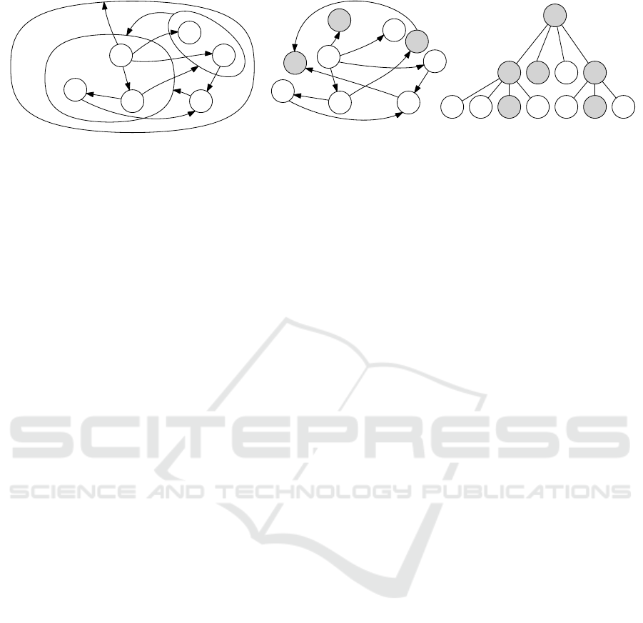
Figure 1: Example of a compound graph

(a) and the corresponding clustered graph

C = (G,T )

(b). The inclusion edges in

(a) are represented by inclusion of the vertices. The representative vertices in

as well as the cluster nodes in

are shaded.

Note that edges of G only connect leaves of T .

containment, it would be difﬁcult to draw adjacency

edges between descendants and ancestors. Hence we

attach in

to each non-leaf vertex

an addi-

tional child

, called representative vertex of

, and

reconnect all edges in

originally incident to

instead. What we obtain now is a clustered graph

C = (G, T )

consisting of the modiﬁed adjacency graph

as the graph

and the inclusion tree

T = D

, whose

leaves are now exactly the vertices of

; see Fig. 1 for

an example, where Fig. 1b shows the clustered graph

corresponding to the compound graph from Fig. 1a.

Throughout the rest of this paper we use this clustered

graph

as the representation of the software structure;

we refer to C as the hierarchic software graph.

The inclusion tree

T = (N,I)

consists of a set of

nodes

N = {µ

,.. . , µ

} ∪V

and the set of inclusion

edges

, where each

is an internal node and each

v ∈ V

is a leaf. We further deﬁne for each node

µ ∈ N

the set

⊂ V

of leaves in the subtree of

rooted at

. Let

be an internal node of

. Then we deﬁne the

local graph

= (V

)

to be the graph with

vertex set

= {ν ∈ N | (ν,µ) ∈ I}

consisting of all

children of

and edge set

= {(ν, η) | ∃u ∈

,v ∈ L

,(u,v) ∈ E}

consisting of all edges induced

by the descendants of V

in the adjacency graph.

Our drawing convention for visualizing hierarchic

software graphs is as follows. We represent each node

(including the leaves) as a disk. Edges of

are

represented as (polygonal) curves connecting the disks

of their endpoints. For simplicity, we identify vertices

and edges with their corresponding disks and curves.

Edges of

are represented by containment, i.e., for

every internal node

, we require that all its children

are positioned inside the disk representing

. We fur-

ther require that no two disks overlap properly or, in

other words, that any two disks are either disjoint or

one is contained in the other. For the adjacency edges

we demand that they do not pass through node disks

(of course they may enter them if their destination is

positioned inside). Our optimization criteria are that re-

lated vertices should be positioned close to each other

and that edge crossings should be avoided. To facilitate

the latter, we bundle edges with similar source or des-

tination into channels that are routed together similar

to micro/macro layouts (Baur and Brandes, 2008).

3 ALGORITHM

Our algorithm follows a two-phase approach. In the

ﬁrst phase, vertex and node placement, we perform

a bottom-up traversal of the hierarchy and determine

for each vertex of the graph and for each node of the

hierarchy a corresponding disk. It ensures that disks

are properly nested according to the inclusion edges.

In the second phase, edge routing, we draw the

edges. We ﬁrst decompose every edge into segments,

each connecting either a child and a parent in the hier-

archy or two siblings. Each segment is associated with

a weight describing how many edges contain it. We

then draw the segments as thick corridors (or channels)

using a geometric heuristic to route around obstacles,

e.g., non-incident vertices. Crossing segments that

share a common endpoint are merged into a larger

segment to avoid crossings. Afterwards, we draw the

actual edges inside the corresponding channels.

3.1 Vertex and Node Placement

For the vertex and node placement we perform a

bottom-up traversal of the cluster tree

. For each

cluster

, we assume that its children

are already

represented by disks

. We assume that the leaves

are represented by disks of a ﬁxed size. When process-

ing an inner node

, our goal is to arrange the disks

representing the children of

in such a way that

(i) they do not overlap, (ii) children that are adjacent

are close to each other, and (iii) the size of the

smallest enclosing disk of the arrangement centered

at the representative vertex

is as small as possible

(over all arrangements of the disks D

To meet these requirements, for any two vertices

and

whose corresponding disks have radius

and

Software Visualization via Hierarchic Micro/Macro Layouts

157

a) b)

Figure 2: Illustration of channel routing. a) Offsetting channels at common ports. b) Reducing overlaps by adding bend points;

iterating results in smooth routing around nodes.

, we deﬁne an offset function

off(u,v) = c

min

min{r

} + c

max

max{r

}, (1)

where

min

max

≥ 0

with

min

+ c

max

= 1

control the

weighting of the smaller and the larger disk radius. To

avoid overlaps, we require that the center points of

and D

have distance at least

min

(u,v) = r

+ r

+ b

min

· off(u,v), (2)

where

min

≥ 1

is a weighting parameter controlling

the amount of white space between the nodes. To

ensure that adjacent disks are close together, we deﬁne

for adjacent nodes u and v a preferred distance

pref

(u,v) = r

+ r

+ b

pref

· off(u,v), (3)

where

pref

≥ b

min

controls the preferred distance of

adjacent vertices. The values

min

and

max

allow a

better control of white space in case the two disks have

very different radii.

Let

denote the corresponding arrangement of

. We then ﬁx the radius of the disk

representing

to be slightly larger than the radius of the smallest

enclosing disk of

centered at a central node in the

graph, i.e., a node with small distance to all other

nodes. Once the whole tree

has been processed, the

ﬁnal arrangement of disks is obtained from the root

drawing

(

is the root of

) by iteratively replacing

the interior of disks

representing non-leaf nodes

by the corresponding arrangement Γ

For computing the layouts of the

, we ﬁrst com-

pute an initial arrangement by taking a maximum

weight spanning forest of

(edges are weighted by

the corresponding number of edges of

) and using a

radial tree layout. This avoids node overlaps in the ini-

tial drawing. Afterwards, we reﬁne the vertex position-

ing using the force-directed algorithm of Fruchterman

and Reingold (Fruchterman and Reingold, 1991) with

some simple modiﬁcations to the forces so that disk-

shaped vertices of non-zero size are handled correctly.

In particular, we use strong repulsive forces to ensure

the minimum distance

min

(u,v)

for all pairs

{u,v}

nodes, and attraction forces for adjacent vertices

{u,v}

whose distance is larger than

pref

(u,v)

. For practical

purposes we found that

min

= 0.05

and

max

= 0.95

with

2 ≤ b

min

≤ 6

and

pref

= 2b

min

gives good results;

see (Schuhmacher, 2015) for more details.

3.2 Edge Routing

Let

and

be two disjoint disks. We deﬁne the

segment

s(D,D

)

connecting

and

as the line seg-

ment between the intersections of the boundaries of

and

and the straight-line segment connecting their

centers. We consider points as disks of radius 0.

We would like to draw the edges as polygonal

curves as follows. For an edge

(u,v)

let

de-

note the lowest common ancestor of

and

let

and

denote the children of

whose subtrees

contain

and

, respectively. We ﬁrst draw the seg-

ment

s(D

)

and denote its endpoints as two ports

and

lying on the respective disk boundaries. It

remains to draw two polygonal curves between

and

as well as between

and

. This can be done

independently of each other. We describe the curve

between

and

, the other curve is constructed anal-

ogously. Let

u = ν

,.. . , ν

= ν

be the unique path

between

and

. We abbreviate the disk

. We deﬁne the port

to be

and iteratively

obtain

i−1

as the port of

s(p

i−1

)

on the boundary

i−1

. The sequence of ports

,.. . , p

deﬁnes the

desired polygonal curve. Linking the three subcurves

yields the polyline for edge

(u,v)

. In the following we

refer to a straight-line segment between two consecu-

tive ports on such a polyline as a segment.

When applying this procedure to all edges, some

segments are encountered multiple times and implic-

itly give rise to edge bundles. We want to avoid over-

plotting by separating overlapping edges. At the same

time, we want to maintain the bundling as it empha-

sizes macro structures of the hierarchic software graph.

To that end, we draw each segment as a thick curve

between its ports, whose thickness is proportional to

the number of edges containing it. We call these thick

curves channels and use them as geometric containers

for drawing in a second step the individual edges with

a ﬁxed pairwise offset.

The ﬁrst step of our drawing procedure performs

the channel routing. Initially, each channel is simply a

thick straight-line segment between its ports. For each

port

the thickness (or size) of the thickest channel at

equals the sum of the sizes of the other channels at

If more than two channels share a port

, we offset the

port positions of the smaller channels such that they

do not overlap, see Fig. 2a. It may still happen that a

IVAPP 2016 - International Conference on Information Visualization Theory and Applications

158

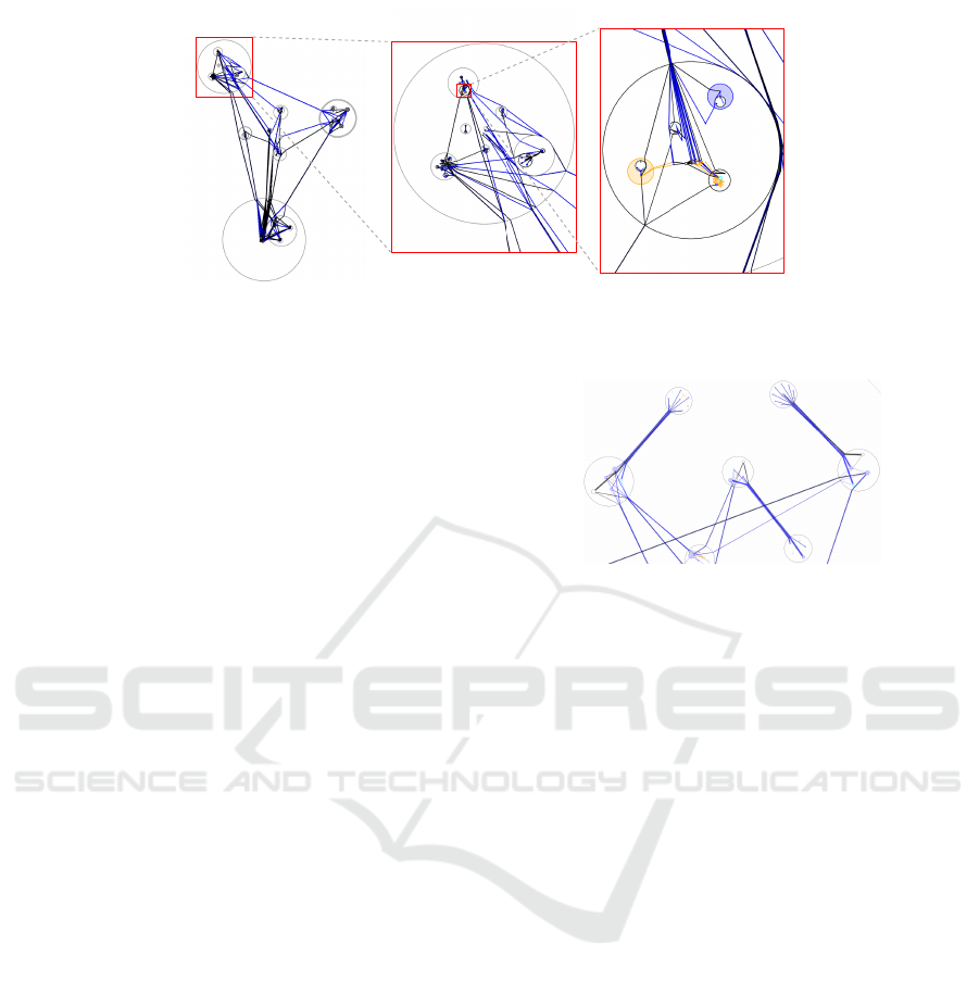
Figure 3: Visualization of a Java software project at three different zoom levels. In the top level, we see the domain model

on the left, the GUI package at the bottom and a utility package in the top right. The middle zoom level shows the internal

structure of the utility package. The lowest level shows the test class of the utility package.

channel crosses non-incident nodes. In order to resolve

such crossings, we iteratively reroute those channels

by introducing an additional bend point and moving it

out of the respective node, see Fig. 2b. This is repeated

until no further improvement is achieved. Finally, we

apply a simple ﬁx to resolve crossings between two

neighboring channels with the same target by merging

them at their ﬁrst intersection into a thicker channel.

The second step routes individual edges within

their induced sequence of channels. In order to avoid

unnecessary crossings within the channels, we use a

simple heuristic to order the outgoing edges at the

vertices of

in a way that reﬂects as much as possible

the hierarchic bundling expressed by the channels.

4 REAL-WORLD EXAMPLES

In this section we present several example visualiza-

tions of real-world software projects. Figure 3 demon-

strates the use of our visualizations for visualizing a

software at different levels of detail. The software

has three main components: a graphical user inter-

face, a domain model and a utility package. The top,

coarsest zoom level gives an overview of the overall

structure and highlights the three main packages (gray

circles) and their relations. The middle view depicts

the internal structure of the utility package. Here, the

bundling inside the channels allows to analyze how

different submodules relate to the external components.

Finally, the bottom, detailed view exhibits the internal

structure of a single class (black circle) composed of

methods (blue disks), constructors (light-blue disks),

ﬁelds (orange disks), as well as some subclasses.

Figure 4 shows a couple of classes and the corre-

sponding test classes. The visualization clearly shows

that each test classes only refers to one class.

Figure 5 shows an example, where by visual inspec-

tion of our layouts we found some code duplication in

a formula parser, which lead to a refactoring.

CursorTest

Cursor

FormulaParserTest

FormulaParser

Figure 4: Visualization of classes and corresponding tests.

5 CONCLUSION

In this paper we have presented a prototype system

for visualizing hierarchical software graphs as mi-

cro/macro node-link diagrams. Our focus in this paper

was the presentation of a tailored algorithm and its pro-

totypical implementation for visualizing hierarchical

compound graphs as they arise in software engineer-

ing. Our current implementation serves as a proof

of concept, but it can already be used to interactively

explore Java software projects. Still, it must be ex-

tended in multiple ways to meet the needs of software

visualization in practice. Thus the next step is to in-

tegrate it into IDEs (e.g., Eclipse) to visually support

software engineering tasks, in particular to enable in-

teractive linking between the visual representations

and the corresponding source code. This includes a

dynamic label placement step that shows the names

of all software entities relevant at the current level of

detail. Figure 7 and Figure 8 show screenshots of a

preliminary integration into Eclipse for a speciﬁc soft-

ware project, which also includes highlighting and a

simple labeling algorithm. Further improvements on

the layout quality comprise additional postprocessing

steps to minimize white space and to improve edge

routing by using smooth curves instead of hard bends

and spreading edges more evenly at vertices.

Once this is done, a more formal validation (Se-

riai et al., 2014) together with software engineers and

Software Visualization via Hierarchic Micro/Macro Layouts

159

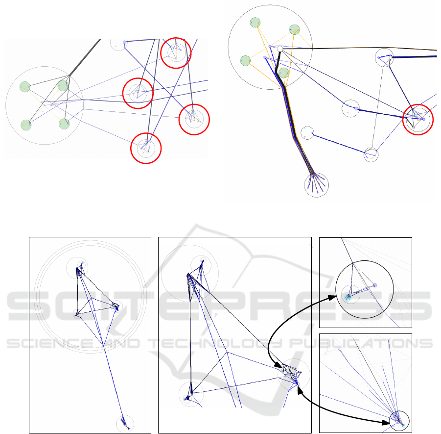
Figure 5: Visualization of a formula parser. The left side visually depicts code duplication (the four marked classes). The right

side shows the same sofware project after a refactoring that removes the code duplication.

GUI

domain model

controller (logic)

main GUI class

GUI element

Figure 6: Visualization of a Java software project (labels have been added manually). The package in the bottom right of the

overview is a utility package. The main package displays very clearly the model view controller architecture of the software.

The top right shows a GUI element (actually a table view). The large node inside represents a subclass used for connecting to

the model. The lower right shows a focus view of the main GUI class, where only the connections of that class are highlighted.

This makes it easy to see that this class references all classes in the GUI package but does not refer to objects outside the GUI

package.

comparison against existing software visualization ap-

proaches is another important step for future work.

REFERENCES

Abuthawabeh, A., Beck, F., Zeckzer, D., and Diehl, S.

(2013). Finding structures in multi-type code couplings

with node-link and matrix visualizations. In Software

Visualization (VISSOFT’13), pages 1–10.

Baur, M. and Brandes, U. (2008). Multi-circular layout of

micro/macro graphs. In Hong, S.-H., Nishizeki, T., and

Quan, W., editors, Graph Drawing, volume 4875 of

Lecture Notes in Computer Science, pages 255–267.

Springer Berlin Heidelberg.

Beyer, D. (2005). Co-change visualization. In Proceedings

of the 21st IEEE International Conference on Software

Maintenance - Industrial and Tool volume, ICSM 2005,

25-30 September 2005, Budapest, Hungary, pages 89–

92.

IVAPP 2016 - International Conference on Information Visualization Theory and Applications

160

Bourqui, R., Auber, D., and Mary, P. (2007). How to

draw clustered weighted graphs using a multilevel

force-directed graph drawing algorithm. In Proc. 11th

Int’l Conference on Information Visualization (IV’07),

pages 757–764. IEEE.

Caserta, P., Zendra, O., and Bodénès, D. (2011). 3d hierarchi-

cal edge bundles to visualize relations in a software city

metaphor. In Visualizing Software for Understanding

and Analysis (VISSOFT’11), pages 1–8. IEEE.

Collberg, C. S., Kobourov, S. G., Nagra, J., Pitts, J., and

Wampler, K. (2003). A system for graph-based visu-

alization of the evolution of software. In Proceedings

ACM 2003 Symposium on Software Visualization, San

Diego, California, USA, June 11-13, 2003, pages 77–

86, 212–213.

Daniel, D. T., Wuchner, E., Sokolov, K., Stal, M., and

Liggesmeyer, P. (2014). Polyptychon: A hierarchically-

constrained classiﬁed dependencies visualization. In

Software Visualization (VISSOFT’14), pages 83–86.

Didimo, W. and Montecchiani, F. (2012). Fast layout com-

putation of hierarchically clustered networks: Algorith-

mic advances and experimental analysis. In Proc. 16th

Int’l Conf. Information Visualization (IV’12), pages

18–23. IEEE.

Diehl, S. (2007). Software Visualization: Visualizing

the Structure, Behaviour, and Evolution of Software.

Springer.

Diehl, S. and Telea, A. C. (2014). Multivariate networks in

software engineering. In Kerren, A., Purchase, H. C.,

and Ward, M. O., editors, Multivariate Network Visual-

ization, volume 8380 of LNCS, chapter 2, pages 13–36.

Springer International Publishing.

Dogrusoz, U., Giral, E., Cetintas, A., Civril, A., and Demir,

E. (2009). A layout algorithm for undirected compound

graphs. Information Sciences, 179(7):980–994.

Frishman, Y. and Tal, A. (2004). Dynamic drawing of

clustered graphs. In Information Visualization (IN-

FOVIS’04), pages 191–198. IEEE.

Fruchterman, T. M. J. and Reingold, E. M. (1991). Graph

drawing by force-directed placement. Software: Prac-

tice and Experience, 21(11):1129–1164.

Holten, D. (2006). Hierarchical edge bundles: Visualiza-

tion of adjacency relations in hierarchical data. IEEE

Transactions on Visualization and Computer Graphics,

12(5):741–748.

Muelder, C. and Ma, K.-L. (2008). A treemap based method

for rapid layout of large graphs. In Proc. IEEE Paciﬁc

Visualization Symposium (PaciﬁcVis’08), pages 231–

238.

Palepu, V. K. and Jones, J. A. (2013). Visualizing constituent

behaviors within executions. In 2013 First IEEE Work-

ing Conference on Software Visualization (VISSOFT),

Eindhoven, The Netherlands, September 27-28, 2013,

pages 1–4.

Patrignani, M. (2013). Handbook of Graph Drawing and Vi-

sualization, chapter Planarity Testing and Embedding,

pages 1–42. Discrete Mathematics and its Applications.

CRC Press.

Ruﬁange, S., McGufﬁn, M. J., and Fuhrman, C. P. (2012).

Treematrix: A hybrid visualization of compound

graphs. Computer Graphics Forum, 31(1):89–101.

Ruﬁange, S. and Melançon, G. (2014). Animatrix: A matrix-

based visualization of software evolution. In Software

Visualization (VISSOFT’14), pages 137–146.

Schuhmacher, A. (2015). Software visualization via hier-

archic graphs. Master’s thesis, Karlsruhe Institute of

Technology (KIT).

Seriai, A., Benomar, O., Cerat, B., and Sahraoui, H. (2014).

Validation of software visualization tools: A system-

atic mapping study. In Software Visualization (VIS-

SOFT’14), pages 60–69.

Sugiyama, K. and Misue, K. (1991). Visualization of struc-

tural information: Automatic drawing of compound

digraphs. IEEE Trans. Syst. Man Cybern., 21(4):876–

892.

van Ham, F. (2003). Using multilevel call matrices in large

software projects. In Information Visualization (INFO-

VIS’03), pages 227–232.

Vehlow, C., Beck, F., and Weiskopf, D. (2015). The state

of the art in visualizing group structures in graphs. In

Borgo, R., Ganovelli, F., and Viola, I., editors, Eu-

rographics Conference on Visualization (EuroVis’15),

STARs.

Wettel, R. and Lanza, M. (2007). Visualizing software sys-

tems as cities. In Proceedings of the 4th IEEE Inter-

national Workshop on Visualizing Software for Under-

standing and Analysis, VISSOFT 2007, 25-26 June

2007, Banff, Alberta, Canada, pages 92–99.

Software Visualization via Hierarchic Micro/Macro Layouts

161

APPENDIX

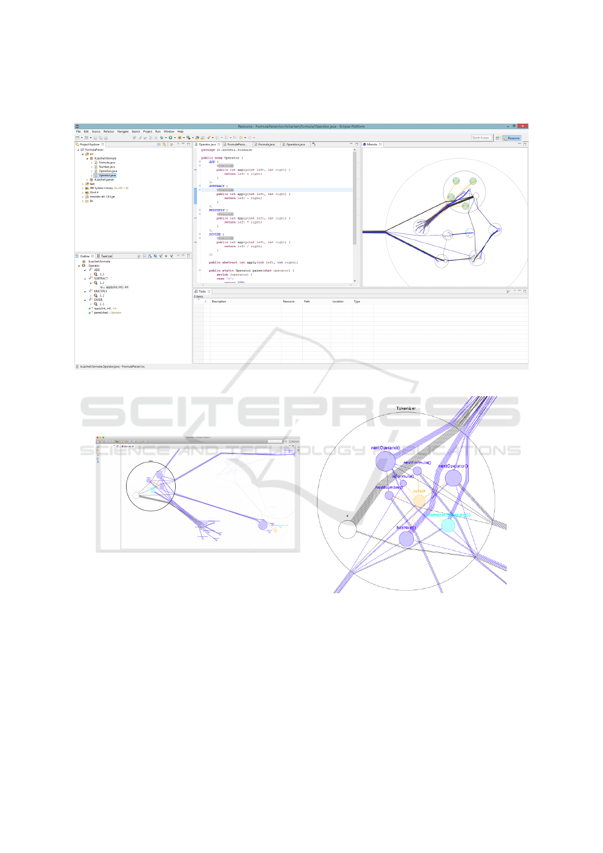
Figure 7: Integration of our visualization into Eclipse for a speciﬁc software project.

Figure 8: The left shows a package in the eclipse integration and highlights only the objects that are referenced from within this

package. The right demonstrates the inclusion of a simple algorithm that labels the entities shown in the visualization.

IVAPP 2016 - International Conference on Information Visualization Theory and Applications

162