
Watch Where You’re Going!
Pedestrian Tracking Via Head Pose
Sankha S. Mukherjee, Rolf H. Baxter and Neil M. Robertson
Visionlab, Institute of Signal Sensors and Systems, Schools of Engineering and Physical Sciences,
Heriot-Watt University, Edinburgh, U.K.
Keywords:
Deep Learning, Intentional Tracker.
Abstract:
In this paper we improve pedestrian tracking using robust, real-time human head pose estimation in low
resolution RGB data without any smoothing motion priors such as direction of motion. This paper presents
four principal novelties. First, we train a deep convolutional neural network (CNN) for head pose classification
with data from various sources ranging from high to low resolution. Second, this classification network is then
fine-tuned on the continuous head pose manifold for regression based on a subset of the data. Third, we
attain state-of-art performance on public low resolution surveillance datasets. Finally, we present improved
tracking results using a Kalman filter based intentional tracker. The tracker fuses the instantaneous head pose
information in the motion model to improve tracking based on predicted future location. Our implementation
computes head pose for a head image in 1.2 milliseconds on commercial hardware, making it real-time and
highly scalable.
1 INTRODUCTION
Automatic gazing direction estimation has become an
important feature for the application of computer vi-
sion to surveillance and human behaviour inference
(Gesierich et al., 2008). Human head pose is the
most important factor in determining focus of atten-
tion (Langton et al., 2004) and provides important
information for group detection, gesture, interaction
detection, and scene understanding (Henderson and
Hollingworth, 1999).
There remains a significant gap in the current
methods for unconstrained head pose estimation in
low resolution. This work addresses the need for
computing low-resolution gaze estimators without re-
liance on motion priors to smooth the estimate and
presents a demonstrably more robust method using
deep learning. In summary, the main scientific con-
tributions of this paper are: (a) Learning a convolu-
tional neural network for human head pose estima-
tion model in an abstract head space that can infer
parameters heads from low resolution, noisy inputs;
(b) Discriminating between head pose angles from
the input image without other prior information us-
ing multi-label discriminative training using various
loss functions; (c) We report state-of-the art results on
two publicly available datasets when compared to the
(previously) state-of-the-art approaches; (d) Using the
robust head pose estimation we report new tracking
results in an intentional tracking framework. Figure
1 demonstrates the output of our instantaneous head
pose estimator on a typical surveillance dataset.
1.1 Related Work
In visual surveillance the resolution of detected heads
can be very small so head pose is often estimated in
coarse discrete directional bins of the azimuthal an-
gle (Robertson and Reid, 2006). See for example the
eight classification bins used in this paper in Figure 3.
Walking direction is then often used as a smoothing
prior (Benfold and Reid, 2008), which reduces mean
squared error, but also attenuates the pure informa-
tion content of the head pose signal. As shown in Fig
2, an analysis of gazing behaviour in several datasets
demonstrates that most people look where they are
going. However, the cases that are of more interest
are when people deviate from this behaviour (i.e. look
somewhere else), as this information could be useful
for anomaly detection or improving tracking (Baxter
et al., 2015).
To obtain an unbiased classifier we, novelly, esti-
mate head pose from the image alone by learning to
represent human heads using a trained CNN. Blanz
et al. (Blanz and Vetter, 1999) use a generative mor-
phable 3D model of human faces in an abstract face-
Mukherjee, S., Baxter, R. and Robertson, N.
Watch Where You’re Going! - Pedestrian Tracking Via Head Pose.
DOI: 10.5220/0005786905730579
In Proceedings of the 11th Joint Conference on Computer Vision, Imaging and Computer Graphics Theory and Applications (VISIGRAPP 2016) - Volume 3: VISAPP, pages 575-581
ISBN: 978-989-758-175-5
Copyright
c
2016 by SCITEPRESS – Science and Technology Publications, Lda. All rights reserved
575
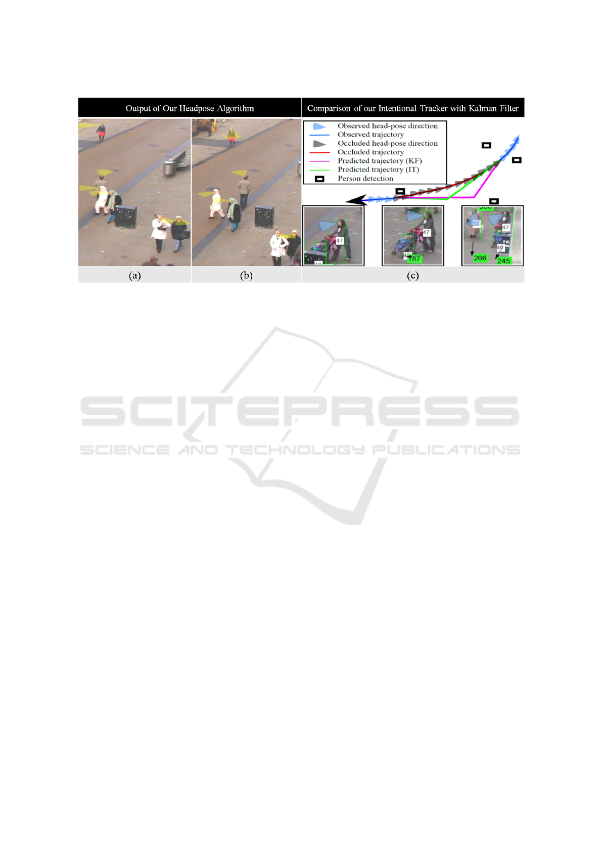
Figure 1: (a) and (b) show the example output of our system showing head pose estimation in the Oxford town centre
dataset(Benfold and Reid, 2011). (c) A real person trajectory/head pose behaviour and predicted trajectory using a Kalman
Filter (KF) and our intentional tracker (IT). Tracking failures can lead to target data association errors. (Bottom) Frames from
the Benfold dataset (Benfold and Reid, 2011) showing pedestrian head pose.
space that can generate human faces with different
shapes, colours and expressions. We learn a repre-
sentation that is valid for human heads under differ-
ent poses and is invariant to expressions, occlusions,
hair, hats, and glasses. CNNs (Szegedy et al., 2014)
have achieved state-of-the-performance in large la-
belled datasets such as the Imagenet.
The pioneering work on low resolution head pose
estimation by Robertson and Reid (Robertson and
Reid, 2006) used a detector based on template train-
ing to classify head poses in 8 directional bins. This
technique was extended to allow colour invariance
by Benfold et al. (Benfold and Reid, 2008), who
proposed a randomized fern classifier for hair face
segmentation before template matching. A few non-
linear regression approaches such as Artificial Neural
Networks (Gourier et al., 2006; Stiefelhagen, 2004)
and high-dimensional manifold based approaches
(Balasubramanian et al., 2007; BenAbdelkader, 2010)
try to estimate the head poses in a continuous range.
These techniques however are more suited to high res-
olution human computer interaction cases where the
head is more or less constrained to near frontal poses.
Chen and Odobez (Cheng and Odobez, 2012) pro-
posed the state-of-the-art method for unconstrained
coupled head pose and body pose estimation in low
resolution surveillance videos. They used multi-level
HOG for the head and body pose features and ex-
tracted a feature vector for adaptive classification us-
ing high dimensional kernel space methods. Coupling
of head pose with such priors results in a head pose
signal that is not very informative: these techniques
perform very well in the range indicated in Figure 2,
but perform poorly when the head pose is not aligned
to the priors. We stress this point because it is impor-
tant for the head pose estimation to provide robust in-
formation that can be further exploited (e.g. improv-
ing tracking, anomaly detection, group detection, be-
haviour analysis) and achieving this goal is what this
paper demonstrates.
Baxter et al. showed that by incorporating head
pose signal into a basic tracker this significantly im-
proves tracking in presence of occlusions and/or bad
detections(Baxter et al., 2015). This method, also
known as intentional tracking, sees significant perfor-
mance gains from having better head-pose estimation.
We propose a more robust head pose estimation com-
pared to their approach and achieve state-of-the-art in
intentional tracking.
2 DEEP LEARNING OF
LOW-RESOLUTION GAZING
ANGLES
In this paper we adapt the the output of any head de-
tector and normalize the heads to 256 × 256 as in-
put to our algorithm. These inputs are then used
to train a CNN. These models belong to a class of
fully supervised deep models that have proven to
be very successful in a wide variety of tasks. The
power of CNNs lie in the ability to learn multiple
levels of non linear transforms on the input data us-
ing labeled examples through gradient descent based
optimizations. The basic building blocks of CNNs
VISAPP 2016 - International Conference on Computer Vision Theory and Applications
576
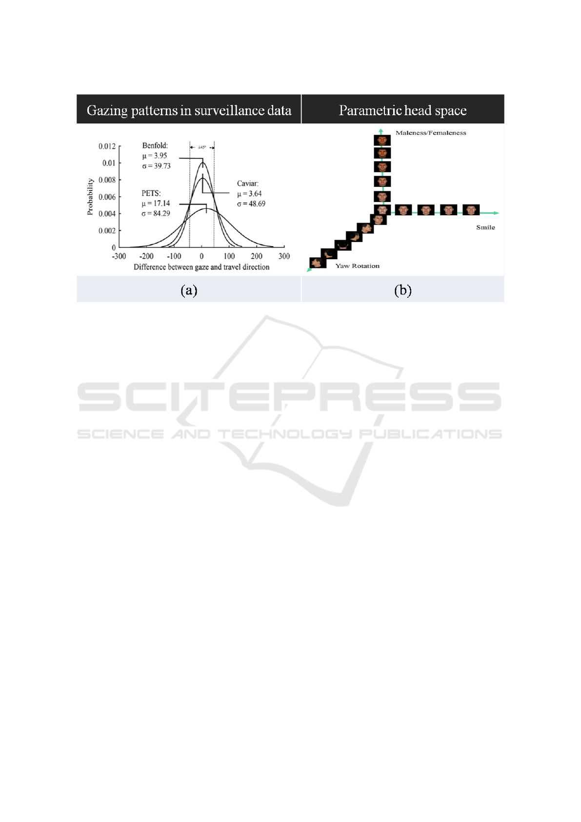
Figure 2: (a) Head pose deviation from walking direction as a Probability Density Function in various datasets (Baxter et al.,
2015) (b) The conceptual parametric human head space.
are fully parameterized (trainable) convolution fil-
ter banks that convolve the input to give feature
maps, non-linearities (like sigmoid or Rectified Lin-
ear Units), pooling layers/downsampling layers (e.g.
max pooling, mean pooling etc.) that down-sample
the feature maps, and fully connected layers. CNNs
in particular through their multiple levels of convolu-
tion and pooling achieve a high degree of translation
invariance in their features. Recent studies from the
VGG group (Simonyan and Zisserman, 2014) have
shown that deeper models with smaller filters achieve
great expressive power in terms of learning power-
ful features from data in tasks like object recognition
on large scale datasets like the Imagenet (Ioffe and
Szegedy, 2015). As the model go deeper the num-
ber of weights/ parameters or the networks grow sig-
nificantly. It then becomes imperative to use large
scale labelled training data to train these networks.
However one should note that the number of param-
eters in the convolution layers are orders of magni-
tude lower than the fully connected layer (Krizhevsky,
2014). Hence by having more convolution layers
helps alleviate the problem of this parameter explo-
sion while retaining the expressive properties on the
deep models. One such model is the recently intro-
duced Googlenet model (Szegedy et al., 2014).
We train a CNN on the RGB data based on this
architecture (Szegedy et al., 2014). This architec-
ture has the state-of-the-art results on the Imagenet
dataset (Ioffe and Szegedy, 2015). In our experiment
the same network also gave the best results on our
task. The advantage of this network lies in that it is
very deep but has a lot less parameters (around 5 mil-
lion) compared to other contemporary networks like
the VGG-16 (Simonyan and Zisserman, 2014) which
has more than 140 million parameters. This lets us
train the networks using considerably less training
data. We improved the network by changing the Rec-
tified Linear Unit non-linearities (RELU) with Para-
metric Rectified Linear Unit and their corresponding
weight initialisation introduced in (He et al., 2015).
The non-linearities are defined as follows
RELU (x) =
(
x i f x > 0
0 i f x ≤ 0
, PRELU (x) =
(
x i f x > 0
mx i f x ≤ 0
(1)
where m, the slope in the negative x is a learn-able
free parameter.
The reason the PRELU activations are better than
their RELU counterpart lies in the fact that PRELU
activations have non zero outputs and non zero gradi-
ents in the negative values. This makes them easier to
propagate gradients for. Whereas in RELUs if the out-
put of a neuron becomes less than zero, its gradients
also vanish and it hampers learning through gradient
descent. The motivation for doing it is that this small
change, without increasing the number of parameters
of the network significantly actually improves the ac-
curacy as shown in (He et al., 2015).
We also exploit the ability of CNNs to learn from
multiple types of labels for the same kind of under-
lying data to achieve a valid representation learnt on
the data. Since there are few explicit head-pose re-
gression datasets, we initialize the training of models
Watch Where You’re Going! - Pedestrian Tracking Via Head Pose
577

Figure 3: Linear Discriminant Analysis (LDA) projected scatter plot of: (a) The classification network features; (b) The
network fine-tuned on regression manifold with a colour map that spans the range 0-360 degrees. Interestingly, the features
maintain the latent circular head pose manifold.
with classification into 8 head pose classes spanning
360 degrees. The representative head-pose classes are
shown in Figure 3. We learn an initial representation
that is then transferred to the regression network and
fine tuned for regression. Figure 3 also shows how
the CNN features separate easily in only two dimen-
sions (it is in reality a much higher dimension feature
space).
For regression we expect to see a similar distribu-
tion that is more evenly spread out on the manifold
instead of forming clusters. Figure 3 shows the out-
put scatter plot of the first two LDA components of
our fine-tuned features on regression on our dataset.
3 INTEGRATING INTENTIONAL
PRIORS IN A KALMAN FILTER
The Regression output is then used as input to a
Kalman Filter (KF) based intentional tracking frame-
work that we now discuss. We fuse intentional priors
into the KF, firstly, by calculating the strength of the
prior, denoted ˆs
t
, using the absolute magnitude of the
deviations for the last 10 time steps (arbitrarily cho-
sen). This allows ˆs
t
to combine both the magnitude
and persistence of the prior signal. The signal strength
at time t is then calculated as follows (where θ
g
k
is the
head pose direction and θ
v
k
is the direction of travel):
ˆs
t
= |
t
∑
k=t−10
θ
g
k
− θ
v
k
| (2)
Next, we weight the influence of the prior. Intu-
itively, the weight (α
t
) should increase in line with
the strength of the prior ˆs
t
. A sigmoid function ap-
plied to ˆs
t
is a simple and effective way to achieve
this. The sigmoid is parameterised by ρ and τ and
could be optimised for the scene to reflect the relia-
bility of the prior, where ρ adjusts the rate at which
the function moves from zero to one and τ adjusts the
’base-weight’ (weight given for zero strength). Rather
than optimising for any particular scene, we use val-
ues for ρ and τ that were empirically derived in (Bax-
ter et al., 2014).
α
t
= (1 + exp(−ρ(ˆs
t
− τ)))
−1
(3)
Having determined α
t
, the transition model (F
t
) is ad-
justed to reduce the influence of the target’s previous
motion. Denote F
t−1
as the motion model at time t −1
and γ
t
= 1 − α
t
. The motion model is then updated as
follows:
F
t
=
1 0 γ
t
0
0 1 0 γ
t
0 0 1 0
0 0 0 1
(4)
This has the effect of reducing the influence of ˙x and
˙y by a factor of γ
t
during the prediction step of the
algorithm. The influence of the intentional prior is
asserted using the control matrix B
t
:
B
t
= [α
t
dx,α
t
dy, α
t
dx,α
t
dy]
T
(5)
dx = d
t
cos(θ
p
),dy = d
t
sin(θ
p
) (6)
Where d
t
is the geometric distance travelled by the
target between t − 1 : t and θ
p
is the predicted travel
direction based on head pose angle θ
d
t−1
. Two ap-
proaches could be used for calculating d
t
: It could
be estimated from [ ˙x
t−1
, ˙y
t−1
], which is an estimate of
VISAPP 2016 - International Conference on Computer Vision Theory and Applications
578

Figure 4: The benefit of headpose as a prior is clearly illustrated when no prior tracking information is available. The Kalman
filter output is shown in red and the intentional tracker output is shown in green. We initialize the tracker with very few frames
and let the trackers evolve without further detection. (a) The person does not cross the road and his headpose at the instant
of exiting the door is very indicative. (b) Similarly for people who want to cross the road, the head pose information is again
very indicative of their intention. There is a region of occlusion that is shown in orange. The trajectories qualitatively show
the benefit of the intentional tracker.
the target’s velocity given observations z
0:t
. Alterna-
tively, a smoothed velocity could be calculated from
[pos
x
t−k:t−1
, pos
y
t−k:t−1
], where 2 ≤ k ≤ t. In practice
the second approach was found to give better perfor-
mance using empirically derived k = 5.
Having finally defined all of the components re-
quired to generate F
t
, the remainder of the KF algo-
rithm remains the same. Predictions are now based
on a target’s previous motion (with weight γ
t
) and the
intentional prior (with weight α
t
).
Furthermore, the instantaneous head pose prior
can be used to initialize tracking where no prior track-
ing information is available. This can be used to ap-
proximately predict pedestrian intent with a few time
steps. Figure 4 shows this scenario qualitatively. It
can be clearly seen that the estimated head pose for
people coming out of the door near the zebra crossing
can be very informative in predicting their intended
action.
4 EXPERIMENTS AND
VALIDATION
We use multiple datasets to train our system and we
validate our approach on two public datasets as dis-
cussed below. We have generated a dataset using the
Kinect and Kinect 2 sensors where we recorded 46
people (32 males, 14 females) freely moving around
with various head-poses in front of the sensor. To get
accurate head pose ground truth data we used a dis-
creet (actually hidden) wearable miniature X-BIMU
IMU sensor which provides the head orientation as a
quaternion. We then recorded each individual for one
minute moving in the field of view with varying dis-
tance (2-8m). We annotated the head in each frame
and associated the IMU data with it in each frame.
We acquired around 1500 frames for each person giv-
ing a dataset of the order of 68000 training examples.
To maximise the training corpus, we gathered data
from multiple sources that had similar underlying dis-
tributions. Datasets annotated for unconstrained face
recognition, facial landmark detection, expression de-
tection all have facial data under various poses. The
different head pose datasets that we used are the Ox-
ford town centre dataset (Benfold and Reid, 2008),
the BIWI Kinect head-pose dataset (Fanelli et al.,
2013), the Caviar shopping centre dataset (htt, ), the
HIIT Head Orientation dataset along with the IDIAP
head-pose dataset (Tosato et al., 2013). It should be
highlighted that the different datasets have different
annotations; some of them have real-valued ground
truth, others have 6-8 classes spanning the 360
◦
. The
datasets also vary in resolution from very high (BIWI)
to very low (Caviar). For regression we use our, Biwi
and the Oxford datasets which have continuous labels.
4.1 Training
For training and validation we split the dataset in a
ratio of 70:30 randomly across several trial runs and
averaged the mean squared error. For training we used
a dropout rate of 20% on before every fully connected
layer. We jittered the input images by mirroring them
(with corresponding change in ground truth) scaling
the bounding box and cropping them with scales 0.75,
0.9, 1.5, 1.8, 2.0 , and 2.5. For all scales greater than
1, we also translated the images randomly by 20%
in both directions. This was done to improve scale
invariance along with mitigating the effects of badly
Watch Where You’re Going! - Pedestrian Tracking Via Head Pose
579

Figure 5: (a) The comparison of our method with the previous best results in terms of mean squared error on the Oxford
dataset(Benfold and Reid, 2011). The Confusion matrices showing the output of: (b) Our classification method on the Oxford
town centre dataset; (c) Our classification on the Caviar dataset.
aligned/ partially occluded head detections. We used
a modified version of the deep learning framework
Caffe (Jia et al., 2014) to train our network.
5 RESULTS
We first validate our CNN based head pose estima-
tion approach on the surveillance datasets and then
show improved tracking results using the intentional
tracker.
5.1 Headpose Estimation Results
For the low resolution surveillance domain dataset,
we report our results on the Oxford and the Caviar
datasets. In these datasets we classify the head pose
into 8 equally spaced (45
◦
) angular bins as shown in
Figure 3. For comparison with (Cheng and Odobez,
2012) and Benfold (Benfold and Reid, 2011) we use
the Oxford dataset in which both have reported re-
sults. One consideration has to be made while com-
paring because (Cheng and Odobez, 2012) reported
the mean square error (MSE) which they derived from
a weighted combination of their 8 class classifier out-
put multiplied with the bin angles as
∑
8
i=1
p
i
−→
η
θ
i
where
p
i
is the classifier output value for the class i and
−→
η
θ
i
is the unit vector in that angular direction. Fig-
ure 5 shows the comparison between our method with
the previous state-of-the-art results. In terms of MSE
we have achieved the best published results. On the
Caviar dataset we achieve 91.2% classification accu-
racy which to our knowledge is the best result on the
dataset. We also present the confusion matrices on
the Oxford and Caviar datasets based on our classifi-
cation network, as shown in Figure 5. On the Ben-
fold dataset our 8 class classification achieves 89.6%
Figure 6: Comparative improvement of our headpose esti-
mation based intentional tracking vs the method of (Baxter
et al., 2015).
accuracy, which again is the highest accuracy of any
technique.
5.2 Tracking Results
We report the cumulative log likelihood (CLL) as our
evaluation metric for direct comparison with (Bax-
ter et al., 2015). CLL is based on the measurement
innovation and is defined as CLL
KF
=
∑
T
k=1
LL
KF
k
and CLL
IT
=
∑
T
k=1
LL
IT
k
. Improvement in CLL is:
CLL
KF
/CLL
IT
. CLL measures how well the inno-
vation covariance is modelled and is a useful metric
when MSE cannot be calculated. We use the same
values for the parameters.
As can be seen from Figure 6, the intentional
tracking performance is greatly improved by better
headpose estimation. On the Benfold dataset we
achieve a CLL median of 8.8% compared to the 5.9%
achieved by their headpose estimation method. Sim-
ilarly, on the Caviar dataset we achieve a CLL me-
dian of 16.02% compared to the 15.8% achieved by
the competing system. It should be noted that on
VISAPP 2016 - International Conference on Computer Vision Theory and Applications
580

Caviar data, the head pose ground truth annotation
based tracker gives a median CLL improvement of
only 16.1% so there is very little room at the top.
However in both the datasets we achieve state-of-the-
art tracking performance.
6 CONCLUSION AND FUTURE
WORK
In this paper we presented a data-driven to low
resolution head pose estimation in the wild. We
achieved state-of-the-art results on two publicly avail-
able datasets. The model fine tuned on head pose re-
gression was able to achieve state-of-the-art perfor-
mance on intentional tracking.
REFERENCES
Caviar dataset. http://homepages.inf.ed.ac.uk/rbf/CAVIAR/.
Balasubramanian, V., Ye, J., and Panchanathan, S. (2007).
Biased manifold embedding: a framework for person-
independent head pose estimation. In Proceeding of
the IEEE Conference on Computer Vision and Pat-
ternRecognition, pages 1–7.
Baxter, R., Leach, M., Mukherjee, S., and Robertson, N.
(2015). An adaptive motion model for person tracking
with instantaneous head-pose features. Signal Pro-
cessing Letters, IEEE, 22(5):578–582.
Baxter, R. H., Leach, M., and Robertson, N. M. (2014).
Tracking with Intent. In Sensor Signal Prcoessing for
Defence.
BenAbdelkader, C. (2010). Robust head pose estimation
using supervised manifold learning. In Proceeding of
the 11th European Conference on Computer Vision,
pages 518–531.
Benfold, B. and Reid, I. (2008). Colour invariant head pose
classification in low resolution video. In Proceeding
of the British Machine Vision Conference.
Benfold, B. and Reid, I. (2011). Unsupervised learning of
a scene-specific coarse gaze estimator. In Computer
Vision (ICCV), 2011 IEEE International Conference
on, pages 2344–2351.
Blanz, V. and Vetter, T. (1999). A morphable model for
the synthesis of 3d faces. In Proceedings of the 26th
Annual Conference on Computer Graphics and Inter-
active Techniques, SIGGRAPH ’99, pages 187–194,
New York, NY, USA. ACM Press/Addison-Wesley
Publishing Co.
Cheng, C. and Odobez, J. (2012). We are not contortionists:
Coupled adaptive learning for head and body orien-
tation estimation in surveillance video. In Computer
Vision and Pattern Recognition (CVPR), 2012 IEEE
Conference on, pages 1554–1551.
Fanelli, G., Dantone, M., Gall, J., Fossati, A., and Van Gool,
L. (2013). Random forests for real time 3d face anal-
ysis. Int. J. Comput. Vision, 101(3):437–458.
Gesierich, B., Bruzzo, A., Ottoboni, G., and Finos, L.
(2008). Human gaze behaviour during action execu-
tion and observation. Acta Psychologica, 128(2):324
– 330.
Gourier, N., Maisonnasse, J., Hall, D., and Crowley, J.
(2006). Head pose estimation on low resolution im-
ages. In Proceeding of the 1st International Evalua-
tion Conference on Classification of Events, Activities
and Relationships, pages 270–280.
He, K., Zhang, X., Ren, S., and Sun, J. (2015). Delving deep
into rectifiers: Surpassing human-level performance
on imagenet classification.
Henderson, J. M. and Hollingworth, A. (1999). High-
level scene perception. Annual Review of Psychology,
50(1):243–271. PMID: 10074679.
Ioffe, S. and Szegedy, C. (2015). Batch normalization: Ac-
celerating deep network training by reducing internal
covariate shift. CoRR, abs/1502.03167.
Jia, Y., Shelhamer, E., Donahue, J., Karayev, S., Long, J.,
Girshick, R., Guadarrama, S., and Darrell, T. (2014).
Caffe: Convolutional architecture for fast feature em-
bedding. arXiv preprint arXiv:1408.5093.
Krizhevsky, A. (2014). One weird trick for parallelizing
convolutional neural networks. CoRR, abs/1404.5997.
Langton, S., Honeyman, H., and Tessler, E. (2004). The
influence of head contour and nose angle on the per-
ception of eye-gaze direction. Perception & Psy-
chophysics, 66(5):752–771.
Robertson, N. and Reid, I. (2006). Estimating gaze direc-
tion from low-resolution faces in video. In Proceeding
of the 9th European Conference on Computer Vision,
2006, volume 3952/2006, pages 402–415.
Simonyan, K. and Zisserman, A. (2014). Very deep convo-
lutional networks for large-scale image recognition.
Stiefelhagen, R. (2004). Estimating head pose with neural
network-results on the pointing04 icpr workshop eval-
uation data. In Proceedings of the ICPR Workshop on
Visual Observation of Deictic Gestures.
Szegedy, C., Liu, W., Jia, Y., Sermanet, P., Reed, S.,
Anguelov, D., Erhan, D., Vanhoucke, V., and Rabi-
novich, A. (2014). Going Deeper with Convolutions.
ArXiv e-prints.
Tosato, D., Spera, M., Cristani, M., and Murino, V.
(2013). Characterizing humans on riemannian man-
ifolds. IEEE Transactions on Pattern Analysis and
Machine Intelligence, 35(8):1972–1984.
Watch Where You’re Going! - Pedestrian Tracking Via Head Pose
581
