Managing Energy Consumption and Quality of Service in Data Centers

Marziyeh Bayati

epartement d’Informatique, LACL, Universit

e Paris-Est Cr

eteil (UPEC), 61 avenue du G

eral de Gaulle, Cr

eteil, France

Keywords:

Data Center, Discrete Stochastic Process, Energy consumption, Energy Saving, Numerical Analysis, Quality

of Service, Queues, Service Performance, Simulation.

Abstract:

The main goal of this paper is to manage the switching on/off of servers in a data center during time to adapt

the system with incoming trafﬁc changes to ensure a good performance and a reasonable energy consumption.

In this work, the system is modeled by a queue then, an optimization algorithm is designed to manage energy

consumption and quality of service in the data center. For several systems, the algorithm is tested by numerical

analysis under various types of job arrivals: arrivals with constant rate, arrivals deﬁned by an constant discrete

distribution, arrivals speciﬁed by a variable discrete distribution over time, and arrivals modeled by discrete

distributions obtained from real trafﬁc traces. The optimization algorithm that we suggest, adapts and adjusts

dynamically the number of operational servers according to: trafﬁc variation, workload, cost of keeping a job

in the buffer, cost of losing a job, and energetic cost for serving a job.

1 INTRODUCTION

The increasing development of Data Centers is caus-

ing problems in energy consumption. More than 1.3%

of the global energy consumption is due to the elec-

tricity used by data centers, a rate that is increasing,

revealed by a survey conducted in (Koomey, 2011),

which says a lot about the increasing evolution of

data centers. Therefore, to ensure both a good per-

formance of services offered by these data centers and

reasonable energy consumption, a detailed analysis of

the behavior of these systems is essential for design-

ing efﬁcient optimization algorithms to reduce the en-

ergy consumption.

Two requirements are in conﬂict: (i) Switching

on a maximum number of servers leads to less waiting

time and decreases the loss of jobs but requires a high

energy consumption. (ii) Switching on a minimum

number of servers leads to less energy consumption,

but causes more waiting time and increases the loss of

jobs.

The goal is to design better managing algorithms

which take into account these two constraints to mini-

mize: waiting time, loss rate and energy consumption.

Studies like in (Berl et al., 2010; Baliga et al.,

2011; Lee and Zomaya, 2012) show that much of

the energy consumed in the data center is mainly due

to the electricity used to run the servers and to cool

them (70% of total cost of the data center). Thus the

main factor of this energy consumption is related to

the number of operational servers. Many efforts have

focused on servers and their cooling. Works have

been done to build better components, low-energy-

consumption processors, more efﬁcient energy cir-

cuits, more efﬁcient cooling systems (Grunwald et al.,

2000), and optimized kernels (Patel et al., 2003).

(Aidarov et al., 2013) analyze an energy optimiza-

tion strategy for a data center where: (i) job ar-

rivals rate, (ii) service price, (iii) promised Quality

of Service (QoS), (iv) penalty paid by the supplier

if the QoS provided is less than promised, are ﬁxed.

Their objective is to maximize revenues from the ser-

vice provider. The strategy should ﬁnd a balance be-

tween minimizing the penalties, minimizing the cost

of energy, and maximizing the number of served jobs.

They used queues as model and tested their strategy

by simulations.

(Mazzucco and Mitrani, 2012) provide a real test

of an energy optimization strategy. The strategy is to

switch on a number of servers : the more waiting jobs

are observed, the more servers are switched on, and

vice versa. Starting and stopping servers are progres-

sive. This strategy has been tested on the platform

Cloud Amazon EC2 with a cluster of servers. They

have compared their strategy with two other strate-

gies: (i) keeping all servers switched on, (ii) starting

and stopping servers periodically.

(Mitrani, 2013) studies the problem of managing

Bayati, M.

Managing Energy Consumption and Quality of Service in Data Centers.

In Proceedings of the 5th International Conference on Smar t Cities and Green ICT Systems (SMARTGREENS 2016), pages 293-301

ISBN: 978-989-758-184-7

293

a data center to keep a low energy consumption. This

problem is modeled by a queue in which jobs can

leave the system if the waiting time is too long. The

proposed strategy is to consider reserve server groups

that are gradually switched on when the number of

jobs in the buffer exceeds a certain threshold. Sim-

ilarly these server groups are gradually switched off

when the number of jobs in the buffer decreases and

exceeds another threshold. The thresholds are analyt-

ically evaluated using an objective function that takes

into account the parameters of the systems.

(Chase et al., 2001) work on an approach based

on the management of servers based on the supplied

performance. The system continuously monitors its

workload and provides resource allocations by esti-

mating their effects on the performance of the service.

They describe a greedy resource allocation algorithm

to balance supply and demand. Their experimental re-

sults show that the consumption of energy is reduced

by 30%.

(Schwartz et al., 2012) present a theoretical queu-

ing model to ﬁnd a compromise between jobs wait-

ing time and energy consumption where a group of

servers is active all the time and the remaining servers

are activated on request.

In (Bayati et al., 2015) we present, with other co-

authors, a tool to study the trade-off between energy

consumption and performance evaluation. The tool

uses real trafﬁc traces and stochastic monotonicity

property to insure fast computation. Given a set of

parameters that are ﬁxed by the modeler, the tool de-

termines the best threshold based policy.

Our approach differs from these methods by sev-

eral points. First it is numerical rather than analyti-

cal or simulation based. Thus, this paper considers

less regular processes than the for example Poisson

process considered by Mitrani. Note that the Marko-

vian assumptions (Poisson arrivals, exponential ser-

vices and switching times) and the inﬁnite buffer ca-

pacity are not mandatory for this analysis. However,

here, the arrival process is assumed to be stationary

for short periods of time and change between peri-

ods. This allows us to represent for instance hourly or

daily variations of the job arrivals. Real trafﬁc traces

are used to build discrete distributions for the job ar-

rival.

In this paper a data center is modeled by a discrete

time queue with a ﬁnite buffer capacity and with a

time slot equals to the sampling period used to sam-

ple the trafﬁc traces. The job arrivals are speciﬁed by

a discrete distribution. The system is analyzed for a ﬁ-

nite time period (let’s say a day or a week). This time

period is divided into sub-intervals where the batch of

arrivals are supposed constant

We design an optimization algorithm in order to

manage energy consumption and QoS in the data cen-

ter. The cost of the consumed energy depends on the

number of operational servers. The QoS cost depends

on the number of waiting time (which depends on

the number of jobs in the buffer) and the losing rate

(which depends on the number of lost jobs). Every

slot, our algorithm minimizes an objective function

that combines the cost of energy and the cost of QoS,

in order to increase or decrease the number of opera-

tional servers according to trafﬁc variation.

As the model is solved numerically, it is much

faster and more accurate than simulation.

The rest of this paper is organized as follows. At

ﬁrst Section 2 models the system by simple queues.

Then, Section 3 develops an optimization algorithms.

And ﬁnally, Sections 4, 5 and 6 test and analyses nu-

merically some systems.

Subsequently we will try to interpret the tests and

explain the behavior of the system. We will carry out

several tests for various types of arrivals: (i) arrivals

with constant rate, (ii) arrivals deﬁned by an constant

discrete distribution, (iii) arrivals speciﬁed by a vari-

able discrete distribution over time, (iv) and arrivals

modeled by discrete distribution obtained from real

trafﬁc traces.

2 QUEUE MODEL DEPICTION

A discrete time model is considered. The number of

job arrivals is given by a discrete random variable. For

any distribution X, X[i] is the probability of item i.

The following operators deﬁned over distributions are

needed to compute the system evolution:

• δ

is the Dirac function with v ∈ N, deﬁned as:

[i] = 1 if i = v and δ

[i] = 0 otherwise (1)

• Z = X ⊗Y is the convolution of distributions. It is

deﬁned by:

Z[i] =

∑

j=0

X[ j] ×Y [i − j] (2)

• Y = SUB

(X) is the distribution X translated by

constant v. This function corresponds to a sub-

traction on the underlying random variable. It is

deﬁned by:

Y [i] = X[i−v] if i > v > 0 and Y [0] =

∑

i=0

X[i] (3)

• Y = MIN

(X) is the distribution X bounded by

constant b. This function corresponds to a mini-

SMARTGREENS 2016 - 5th International Conference on Smart Cities and Green ICT Systems

294

mum on the underlying random variable. It is de-

ﬁned by:

Y [i] = X [i] if i < b and Y [b] =

∞

∑

i=b

X[i] (4)

Let DC be a data center composed of Max identi-

cal servers working under the FIFO

discipline. DC

receives jobs requesting the proposed service. The

number of jobs served by one server in one slot is

assumed to be constant and denoted by S. The job

arrivals are sampled with a time interval equal to the

slot duration. Thus, the queuing model is a batch ar-

rival queue with constant services and ﬁnite capacity

buffer B (buffer size). The number of jobs arriving to

S × M(t)A(t): job arrivals

B: Buffer size

N(t): Waiting jobs

M(t): Number of operational servers

S: Number of jobs served by a server per slot

Figure 1: Illustration of the queuing model.

the data center during the t

slot is denoted by A(t)

which is a discrete distribution. N(t) denotes the dis-

tribution of the number of waiting jobs in the buffer

(buffer length). The number of operational servers

during the slot t is denoted by M(t). Thus, M(0) is

the initial number of operational servers and Max is

the maximal number of servers which can be oper-

ational. The distribution N(t) can be computed by

induction on t using the previous operators. As a

discrete-time model is considered, the exact sequence

of events during a slot have to be described. First, the

jobs are added to the buffer then they are executed by

the servers. The admission is performed per job ac-

cording to the Tail Drop policy: a job is accepted if

there is a place in the buffer, otherwise it is rejected.

The following equations give the distributions of the

number of waiting jobs in the buffer and the lost jobs.

For t ≥ 1, we have:

N(t) = MIN

(SUB

S×M(t)

(N(t − 1) ⊗ A(t))) (5)

From now it is assumed that N(0) = δ

. The distribu-

tion of the number of the lost jobs during slot t is:

R(t) = SUB

(S×M(t)+B)

(N(t − 1) ⊗ A(t)) (6)

First In First Out.

Thus A(t), N(t) and R(t) are distributions, and M(t) is

an integer value. It is assumed that the input arrivals

are independent of the current queue state and the past

of the arrival process. Under these assumptions, the

model of the queue is a time-inhomogeneous Discrete

Time Markov Chains. The problem we have to deal

with is related to the nature of the arrival process.

Typically, the job arrivals cannot be assumed to be

stationary. The data center adapts to the ﬂuctuation of

the process by changing the number of servers associ-

ated with the queue, such a policy leads to a trade-off

between the performance (i.e. waiting and loss prob-

abilities) and the energy consumption (i.e. number

of operational servers). However, as the number of

servers changes with time, the system becomes more

complex to analyze.

The number of servers may vary according to

the trafﬁc and performance indexes. More precisely,

distributions N(t) and R(t) are considered and then

some decisions are taken according to a particular cost

function. Let t be the current slot, the expectations

E(N(t)) and E(R(t)) are considered.

Other parameters may be considered:

• the latency to switch on or off a server, which is

a discrete non negative integer values, assumed to

be zero in this study.

• the number of servers g that are switched on or

off. It is a discrete positive integer value. During

this analyses we assume that g = 1.

The energy consumption takes into account the

number of operational servers. Each server consumes

some units of energy per slot when a server is opera-

tional and it costs c

monetary unit. The total energy

used is the sum of units of energy consumed among

the sample path.

QoS takes into account the number of waiting and

lost jobs. Each waiting job costs c

monetary unit per

slot. A loss job cost c

monetary unit:

Table 1: Considered costs.

Cost Meaning

energetic cost for running one operational serer during one slot

waiting cost for one job over one slot

rejection cost for one losing one job

3 OPTIMIZATION ALGORITHM

In any optimization problem we have to minimize a

cost or a maximize gain. In our problem we may both:

• Minimize the number of operational servers M(t)

to minimize the cost paid for electricity.

Managing Energy Consumption and Quality of Service in Data Centers

295

• Minimize the number of waiting and lost jobs,

N(t) and R(t), to minimize the waiting time and

the loss rate which increase the QoS.

This section explains our approach to optimize en-

ergy and QoS. Based on some elements of the system

like the number of job arrivals, the number of waiting

jobs, the number of rejected jobs and the number of

servers, the method consists in turning on or off, each

slot, an optimal number of servers to minimize en-

ergy consumption and maximize the QoS. So we will

need to evaluate every slot the number of waiting and

rejected jobs. Notice that parameters M(t) and N(t)

& R(t) are dependent and connected, gain on energy

consumption leads to a degradation on the QoS and

vice versa. Let’s deﬁne the following objective cost

function:

C(t) = c

×M(t)+c

×E(N(t))+c

×E(R(t)) (7)

Knowing the parameters of the system at slot

(t − 1), our strategy consists to determine the best

number of servers to be switched on, in slot t, in order

to minimize the cost. To do so, every slot t: for each

possible value of M(t) ∈ {0, 1, . . . , Max}, we compute

C(t) and then we returns the value of M(t) that mini-

mizes the cost C(t).

Each slot, our algorithm evaluates all possible

costs for switching on any possible number of servers,

then it returns the number of servers for which the

value of the cost is minimal.

Table 2: Example of optimization. Suppose Max = 10, B =

15, S = 3, c

= 11, c

= 5, c

= 0 and for t = 1 we have:

E(N(t − 1)) = 5 and E(A(t)) = 7. In this case our algorithm

chooses M(t) = 4 this value leads to the minimal cost.

M(t) 0 1 2 3 4 5 6 7 8 9 10

C(t) 60 56 52 48 44 55 66 77 88 99 110

Algorithm 1: Optimization for slot t.

1Data: Max, S, B, N

t−1

, A

, c

2Result: M

3cost min ← ∞

4servers min ← 0

5for M ← 0 to Max (by a step of g) do

6N ← MIN

(SUB

S×M

t−1

⊗ A

))

7R ← SUB

(S×M+B)

t−1

⊗ A

)

8cost← c

× M + c

× E(N) + c

× E(R)

9if cost < cost min then

10cost min ← cost

11servers min ← M

12end

13end

14M

← servers min

As in (Bayati et al., 2015), taking into account the

monotonicity of the system and using coupling de-

tection algorithm (Sericola, 1999), numerical analy-

sis becomes faster by avoiding unnecessary computa-

tions.

In the next sections, we will use this optimization

algorithm to test, simulate, analyze and compare the

evolution of cost (energy consumption and QoS) of a

computer center for different types of job arrivals. We

will consider mainly three types of arrivals: (i) Sec-

tion 4 which analyzes constant arrival rate. (ii) Sec-

tion 5 which considers arrivals modeled by an con-

stant distribution. (iii) Section 6 which is addressed to

arrivals modeled by a pairwise constant distribution.

4 CONSTANT ARRIVAL RATE

Let’s ﬁrst study the case where arrivals are modeled

by a constant rate of job arrivals:

a ∈ R : ∀t : A(t) = δ

(8)

Given the variety of parameters that must be taken

into account to test and analyze our optimization, we

deﬁne the workload of the system as follows:

ρ =

E(A)

Max × S

(9)

Table 3: Workload of system according to ρ.

ρ 0.2 0.5 0.7 0.9 1.2

relaxed moderate comfortable high excessive

4.1 Optimization and Workload

Tests show that, our algorithm turns on, eventually, a

number of servers proportional to the system work-

load (see Figure 2). Although our algorithm calcu-

Workload of system ρ

Number of operational servers M(t)

0.0 0.1 0.3 0.4

0.6

0.7 0.8 1.0 1.1 1.3 1.4

Max = 10

Max = 20

Max = 30

Max = 40

Figure 2: Relationship between the number of operational

servers and the system workload.

SMARTGREENS 2016 - 5th International Conference on Smart Cities and Green ICT Systems

296

lates from the beginning the best number of servers

to be switched on, we observed that this number is

kept the same during the whole observation period:

∀t M(t) =

ρ × Max

. This formula is only valid if

the workload of the system ρ is smaller than 1. Other-

wise, if the workload is greater than 1, the best num-

ber of servers to be turned on will exceed the number

of servers available, so the system turns on all avail-

able servers to be as close as possible to the optimal

number of servers. Finally, the number of servers to

be switched on by our algorithm in the case of a con-

stant arrival rate is given by:

∀t : M(t) = min(

ρ × Max

, Max) (10)

Note that the more the system has heavy workload,

the more the number of operational servers is big-

ger. Note that the results of this subsection are true

for costs c

, c

and c

of the same order of magni-

tude. In the next subsection, we will show impact of

varying the order of magnitude between these costs.

4.2 Cost Order Magnitude

For the rest, notice that the value

gives the energy

cost paid in a slot for the treatment of one single job

by a server. The various tests we have done show that

Table 4: Impact of costs on the number of operational

servers.

Condition # operational servers Behavior

>> c

, c

0 Lazy

<< c

, c

Max Fully active

≈ c

, c

min(

ρ × Max

, Max) Proportional

the behavior of our strategy against energy & QoS op-

timization depends on the values

, c

, and c

. We

distinguish mainly three types of behavior:

• If cost

is higher than c

and c

, the system

prefers to turn off all servers because the cost of

switching on a server to serve S jobs is more ex-

pensive than the cost of rejecting and/or keeping S

jobs in the buffer. We say that the system is lazy.

• If cost

is smaller than c

and c

, then the sys-

tem prefers to turn on all the servers because the

total cost of waiting and rejection is much more

important than the cost of the switching on more

servers. We say that the system is fully active.

• If costs

, c

& c

are close to each

other, the system immediately turns on a num-

ber of servers proportional to the workload:

min(

ρ × Max

, Max).

To better clarify the results reported in the table 4 a

closer analysis of the relationship between costs, sys-

tem workload and the optimal number of servers is

discussed in the following.

Theorem 1. Assume that the buffer size is inﬁnite.

For any slot t: M(t) =



Max if

< c

0 otherwise.

Proof. Assume that B is ∞. This implies that all jobs

will be accepted and no job will be rejected, which

means that the number of loss jobs R(t) is always

zero: (B is ∞) =⇒ (∀ t : R(t) = 0). The total cost

C(t) will be:

× M(t) + c

× E(N) +c

× E(R)

× M(t) + c

× E(N) +c

× 0

× M(t) + c

× E(N)

× M(t) + c

× E(MIN

(SUB

S×M(t)

(N(t − 1) ⊗ A(t))))

× M(t) + c

× E(MIN

∞

(SUB

S×M(t)

(N(t − 1) ⊗ A(t))))

× M(t) + c

× E(SUB

S×M(t)

(N(t − 1) ⊗ A(t))).

As A(t) is modeled in this section by a constant rate,

we have: ∀t : A(t) = δ

, we deduce that:

C(t) = c

× M(t) + c

× max{0, N(t − 1) + a − S × M(t)}.

We have two cases:

1. if (N(t − 1) + a − S × M(t)) ≤ 0

then C(t) = c

× M(t).

In this case we must always choose M(t) = 0 to

ensure a minimum total cost.

2. if (N(t − 1) + a − S × M(t)) > 0 then

C(t) =c

× M(t) + c

× (N(t − 1) + a − S × M(t))

= M(t) × (c

− S × c

) + c

× (N(t − 1) + a).

It is clear that the right term c

×(N(t −1)+ a) is

always a positive value. Thus minimizing the to-

tal cost requires the minimization of the left term

M(t) × (c

− S × c

). Thus, we are mainly deal-

ing with two sub-cases:

(a) If

> c

then M(t) × (c

− S × c

) is nega-

tive, and choosing a maximum value of M(t) =

Max assures a minimum total cost.

(b) If

< c

then M(t) × (c

− S × c

) is pos-

itive, and choosing a zero value of M(t) = 0

provides a minimum total cost.

5 CONSTANT ARRIVAL

DISTRIBUTION

In this section we will study the case where arrivals

are modeled by a single constant distribution that does

not change over time: ∀t : A(t) = D.

As in the previous section we have implemented

and tested our method based on the objective function

to test and analyze the behavior of the system. We

will consider three types of job arrival distributions

Managing Energy Consumption and Quality of Service in Data Centers

297

with the same expectations (to keep nearly the same

workload) but with different variances:

• Uniform arrivals: same probability everywhere in

the distribution.

• Middle arrivals: high probabilities in the middle

of the distribution and low probability at the ex-

tremities (leads to low variance).

• Extremities arrivals: low probability in the mid-

dle of the distribution and high probabilities at the

extremities (leads to high variance).

Table 5 illustrates the three types of the considered

distributions.

Table 5: Example of the considered distributions.

Arrivals Type Distribution E(A) Var(A)

Uniform

i [ 0 , 2 , 4 , 6 , 8 ]

A[i] [ 0.20 , 0.20 , 0.20 , 0.20 , 0.20 ]

4 8

High in middle

i [ 0 , 2 , 4 , 6 , 8 ]

A[i] [ 0.05 , 0.20 , 0.50 , 0.20 , 0.05 ]

4 2.4

High at extremities

i [ 0 , 2 , 4 , 6 , 8 ]

A[i] [ 0.40 , 0.08 , 0.04 , 0.08 , 0.40 ]

4 13.44

5.1 Workload Variation

In this subsection we will use the three types of ar-

rivals we have previously introduced to analyze nu-

merically the system whose parameters are described

in Table 6. Figure 3 shows the evolution, over time,

Table 6: Settings of the ﬁrst numerical analysis.

Parameters Value Unit Description

Max 150 servers total number of servers

S 1 jobs/server processing capacity of a server

B 1000 jobs buffer size

E(A) 20-150 jobs average job arrivals

10 e cost of energy needed by a server

12 e cost of waiting a job

11 e cost of rejecting a job

of the number of operational servers according to sev-

eral workload values of ρ. Clearly, on the curves of

this graph, we observe that the number of operational

servers tends progressively to a value proportional to

the system workload. The more the system has heavy

workload, the more the needed operational servers is

bigger. If the system is overwork-loaded the system

eventually turn on all available servers. Thus, in gen-

eral, the ultimate number of operational servers for a

long term converges to: min

{

Max,

ρ × Max

Furthermore, Figure 3 shows that for the same

workload value ρ, the ultimate number of operational

servers is reached quickly for middle arrivals (red

curve), slowly for uniform arrivals (curve blue), and

very slowly for extremities arrivals (orange curve).

Note that the results of this subsection were ob-

tained for close costs (same order of magnitude). In

the following subsection, we will conduct tests by

varying costs c

, c

and c

Time t

Number of operational servers M(t)

8 10 13

18 20 23

28 30 33

38 40 43

105

113

120

128

135

143

150

ρ = 67%

ρ = 74%

ρ = 87%

ρ = 47%

ρ = 20%

Middle arrivals

Uniform arrivals

Extremities arrivals

Figure 3: Evolution, over time, of the number of operational

servers depending on workload values ρ according to sev-

eral type of arrivals.

5.2 Cost Variation

In this subsection we will consider an analysis with a

ﬁxed job arrivals distribution A(t) with a ﬁxed expec-

tation and a ﬁxed variance, where varying the costs

, c

& c

. We analyze numerically the system

whose parameters are described in Table 7.

Table 7: Settings of the second numerical analysis.

Parameters Value Unit Description

Max 300 servers total number of servers

S 1 jobs/server processing capacity of a server

B 1000-9000 jobs buffer size

E(A) 155 jobs average job arrivals

Var(A) 149.92

jobs variance in job arrivals

ρ 52% - workload

5.2.1 Loss Cost

In this numerical analysis we have set a small value

for the cost of energy consumption

and even

smaller value for the cost of waiting c

but a high

value for the cost of rejection c

: c

> c

We observe that at the beginning and during a cer-

tain period, the system keeps all the servers switched

off and holds jobs on waiting, because the cost of

turning on a server is higher than keeping a job wait-

ing. Thus the system prefers to put jobs on buffer.

That said, after a certain latency period the buffer B

becomes full and the system begins to reject jobs, and

as the loss cost is too high compared to other costs,

the system starts to turn on servers in order to reduce

loss rate. Figure 4 illustrates this reaction latency phe-

nomenon. Curves show that the larger the buffer B is,

the longer latency period is. Therefore, the latency

period before the response of the system can be ap-

proximated by:

E(A)

. Now, ﬁxing B the size of the

buffer and varying c

(while keeping c

> c

SMARTGREENS 2016 - 5th International Conference on Smart Cities and Green ICT Systems

298

Time t

Number of operational servers M(t)

29 34 39 44 49

54 59 64 69

74 78 83 88 93 98

106

115

124

133

142

150

159

168

177

B = 1000

B = 5000

B = 7000

B = 9000

Figure 4: Latency phenomenon.

We observe that the system period latency is the same

(because the value of B was ﬁxed) for the different

values of c

. However, the higher the cost c

is, the

higher the system turns on servers. It is a completely

natural reaction because the system tries to minimize

the total cost, and as the loss cost c

is highest, the

system will turn on more servers to serve more jobs

and emptying further the queue which allows a low

loss rate. Figure 5 illustrates this phenomenon.

Time t

Number of operational servers M(t)

29 34 39 44 49

54 59 64 69

74 78 83 88 93 98

102

111

119

128

136

145

153

162

170

= 1.65

= 1.95

= 3.15

= 6.15

Figure 5: Evolution of the number of operational servers for

different values of loss cost c

5.2.2 Waiting Cost

In this subsection we have set a small value for the

cost of energy consumption

and a high value for

the cost of waiting c

with any value for the loss

cost. Figure 6 illustrates the result of this conﬁgura-

tion. We observed that from the beginning, the system

switch on a signiﬁcant number of servers because the

cost of energy is lower than the one of waiting. Thus

the system prefers to turn on more servers to serve

more jobs and avoid long waiting time. Eventually,

we note that the loss cost is not involved in this con-

Time t

Number of operational servers M(t)

0 2 3

5 6

8 9 11 12 14

17 19 20 22 23

25 26

28 29 31

109

124

140

155

171

186

202

217

233

248

264

279

295

310

= 1.50

= 1.90

= 2.30

= 3.50

Figure 6: Evolution of the number of operational servers for

different values of waiting cost c

ﬁguration, because the system is fairly active and loss

rate is negligible.

6 VARIABLE ARRIVAL

DISTRIBUTION

In this section we will generalize our study extending

it for arrivals modeled by a distribution that changes

over time: ∃t

∃t

: A(t

) 6= A(t

6.1 Hourly Arrival Variation

In a real data center the arrivals jobs vary over the day.

For example high rate arrivals between 8 a.m. and 4

p.m., low arrivals between 4 p.m. and midnight, and

medium arrivals between midnight and 8 a.m. Fig-

ure 7 shows the results of analyzing numerically the

system whose parameters are described in Table 9.

We observe that the system turns on a number of

servers at the beginning of the day to treat arriving

jobs. Then, it gradually increases the number of op-

erational servers to treat the high arrival rate between

Table 8: Example of hourly variation of arrivals.

Arrivals rate Period A(t) E(A)

Medium arrivals 0 a.m.-8 a.m.

i [ 0 , 100 , 200 , 300 , 400 , 500 ]

A[i] [ 0.48 , 0.24 , 0.12 , 0.08 , 0.04 , 0.04 ]

100 jobs

High arrivals 8 a.m.-4 p.m.

i [ 0 , 100 , 200 , 300 , 400 , 500 ]

A[i] [ 0.17 , 0.04 , 0.13 , 0.17 , 0.22 , 0.27 ]

300 job

Low arrivals 4 p.m.-0 a.m.

i [ 0 , 100 , 200 , 300 , 400 , 500 ]

A[i] [ 0.73 , 0.15 , 0.07 , 0.03 , 0.01 , 0.01 ]

50 jobs

Table 9: Settings of the third numerical analysis.

Parameters Value Unit Description

Max 400 servers total number of servers

S 1 jobs/server processing capacity of a server

B 3000 jobs buffer size

7 e cost of energy needed by a server

9 e cost of waiting a job

8 e cost of rejecting a job

Managing Energy Consumption and Quality of Service in Data Centers

299

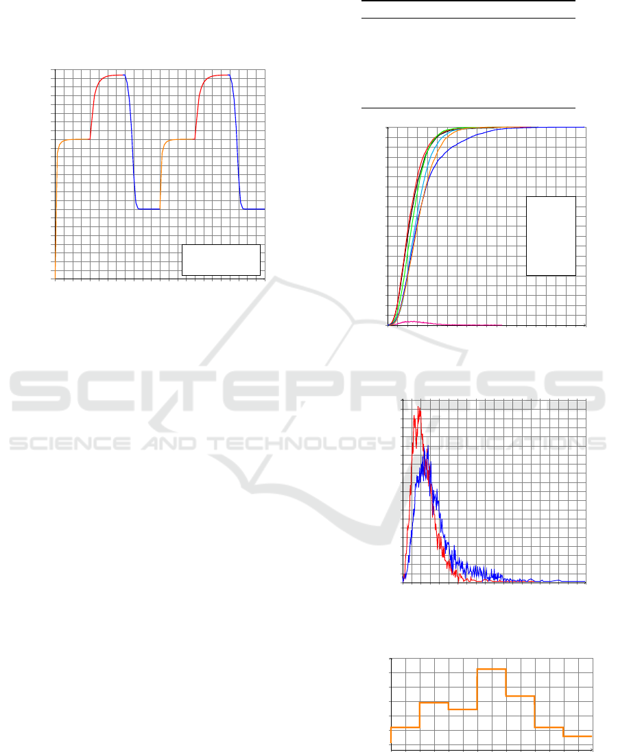
8 a.m. and 4 p.m. Then from 4 p.m. it begins to turn

off the servers and keeping only reduced number of

operational servers to serve the low arrival rate until

midnight. We clearly note the dynamic adaptation of

the energy optimization system to the trafﬁc variation.

Hours

Number of operational servers M(t)

0h 4h 8h 12h

16h

20h 24h 28h 32h

36h

40h 44h 48h

100

113

125

138

150

163

175

188

200

213

225

238

250

263

275

288

300

Medium arrivals

High arrivals

Low arrivals

Figure 7: Evolution of the number of operational servers

during two days.

6.2 Daily Arrival Variation

This section uses real trafﬁc traces to model arrivals.

We use the open clusterdata-2011-2 trace (Wilkes,

2011; Reiss et al., 2011), and we focus on the part

that contains the job events corresponding to the re-

quests destined to a speciﬁc Google data center for

the whole month of May 2011. The job events are or-

ganized as a table of eight attributes; we only use the

column timestamps that refer to the arrival times of

jobs expressed in µ-sec. This trafﬁc trace is sampled

with a sampling period equal to the slot duration. We

consider frames of one minute to sample the trace and

construct seven empirical distributions corresponding

to arrivals during each day of the week. Such an as-

sumption is consistent with the week evolution of job

arrivals observed by long traces.

High arrivals rate is observed on Thursday, low

arrivals rate on Saturday, Sunday and Monday, and

medium arrivals rate during the rest of the week (see

Table 10). These distributions have different statisti-

cal properties reﬂecting the ﬂuctuation of trafﬁc over

the week (see Figure 8). For instance, we observe an

average of 39 (resp. 58) jobs per minute during Sun-

day (resp. Thursday) with a standard deviation of 22

(resp. 38)(see Figure 9). Figure 10 shows the results

of analyzing numerically the system whose parame-

ters are described in Table 11.

Table 10: Example of daily variation of arrivals obtained

from Google traces.

Day of week Arrivals rate E(A) σ(A)

Monday Low 43 jobs 21

Tuesday Medium 51 jobs 25

Wednesday Medium 49 jobs 23

Thursday High 58 jobs 38

Friday Medium 53 jobs 25

Saturday Low 41 jobs 24

Sunday Low 39 jobs 22

Number of jobs

Probability

0 17 33

50 66

83 99

116

132 149

165

182 198

215

231 248

264

281 297 314 330

0.00

5· 10

−2

1· 10

−1

0.15

0.20

0.25

0.30

0.35

0.40

0.45

0.50

0.55

0.60

0.65

0.70

0.75

0.80

0.85

0.90

0.95

1.00

Monday

Tuesday

Wednesday

Thursday

Friday

Saturday

Sunday

Figure 8: Cumulative distribution of A(t) for days of the

week.

Number of jobs

Probability

0 17 33

50 66

83 99

116

132 149

165

182 198

215

231 248

264

281 297 314 330

0.00

1.27· 10

−3

2.55· 10

−3

3.81· 10

−3

5.1· 10

−3

6.36· 10

−3

7.64· 10

−3

8.91· 10

−3

1.02· 10

−2

1.15· 10

−2

1.27· 10

−2

1.4· 10

−2

1.53· 10

−2

1.66· 10

−2

1.78· 10

−2

1.91· 10

−2

2.04· 10

−2

2.17· 10

−2

2.29· 10

−2

2.42· 10

−2

2.55· 10

−2

Figure 9: Distribution of A(t) for Sunday (red curve) and

Thursday (blue curve)

Week days

M(t)

Monday Tuesday Wednesday Thursday Friday Saturday Sunday

Figure 10: Evolution, over a week, of the number of oper-

ational servers. Our algorithm adapts the number of opera-

tional server according to the trafﬁc variation.

SMARTGREENS 2016 - 5th International Conference on Smart Cities and Green ICT Systems

300

Table 11: Settings of the last numerical analysis.

Parameters Value Unit Description

Max 100 servers total number of servers

S 1 jobs/server processing capacity of a server

B 300 jobs buffer size

7 e cost of energy needed by a server

23 e cost of waiting a job

29 e cost of rejecting a job

7 CONCLUSION

In this paper we presented an optimization stochastic

algorithm in order to manage energy consumption and

QoS in a data center modeled by discrete time queue.

Every slot, the algorithm minimizes an objective

function that combines the cost of energy and the cost

of QoS, in order to change the number of operational

servers according to trafﬁc variation.

We show the ability of our algorithm to adapt

dynamically to arrivals changes. Test were showed

through various numerical analysis for several types

of arrivals: (i) arrivals with constant rate, (ii) arrivals

deﬁned by an constant discrete distribution, (iii) ar-

rivals speciﬁed by a variable discrete distribution over

time, (iv) and arrivals modeled by discrete distribu-

tion obtained from Google real trafﬁc traces. The sys-

tem starts turning on servers progressively when high

arrivals rate is detected. And turn off gradually the

servers when arrivals rate becomes low.

Doing a closer analysis of the relationship be-

tween costs, workload and optimal number of oper-

ational servers is considered for future work to de-

termine more accurate link between these parameters.

We also intend to extend this study for the case in

which, the number of served jobs in a slot by a server

is deﬁned by a distribution, the latency to switch on or

off a server is not zero, and the servers are not identi-

cal in performance and energy consumption.

ACKNOWLEDGEMENTS

Special thanks to Vekris, D. and Dahmoune, M..

REFERENCES

Aidarov, K., Ezhilchelvan, P. D., and Mitrani, I. (2013).

Energy-aware management of customer streams.

Electr. Notes Theor. Comput. Sci., 296:199–210.

Baliga, J., Ayre, R. W., Hinton, K., and Tucker, R. S. (2011).

Green cloud computing: Balancing energy in process-

ing, storage, and transport. Proceedings of the IEEE,

99(1):149–167.

Bayati, M., Dahmoune, M., Fourneau, J., Pekergin, N., and

Vekris, D. (2015). A tool based on trafﬁc traces and

stochastic monotonicity to analyze data centers and

their energy consumption. In Valuetools ’15: 9th

international conference on Performance evaluation

methodologies and tools, page to appear. Acm.

Berl, A., Gelenbe, E., Di Girolamo, M., Giuliani, G.,

De Meer, H., Dang, M. Q., and Pentikousis, K. (2010).

Energy-efﬁcient cloud computing. The computer jour-

nal, 53(7):1045–1051.

Chase, J. S., Anderson, D. C., Thakar, P. N., Vahdat, A. M.,

and Doyle, R. P. (2001). Managing energy and server

resources in hosting centers. In ACM SIGOPS Op-

erating Systems Review, volume 35, pages 103–116.

ACM.

Grunwald, D., Morrey, III, C. B., Levis, P., Neufeld, M.,

and Farkas, K. I. (2000). Policies for dynamic clock

scheduling. In Proceedings of the 4th Conference on

Symposium on Operating System Design & Implemen-

tation - Volume 4, OSDI’00, pages 6–6, Berkeley, CA,

USA. USENIX Association.

Koomey, J. (2011). Growth in data center electricity use

2005 to 2010. A report by Analytical Press, completed

at the request of The New York Times, page 9.

Lee, Y. C. and Zomaya, A. Y. (2012). Energy efﬁcient uti-

lization of resources in cloud computing systems. The

Journal of Supercomputing, 60(2):268–280.

Mazzucco, M. and Mitrani, I. (2012). Empirical evaluation

of power saving policies for data centers. SIGMET-

RICS Performance Evaluation Review, 40(3):18–22.

Mitrani, I. (2013). Managing performance and power con-

sumption in a server farm. Annals OR, 202(1):121–

134.

Patel, C. D., Bash, C. E., Sharma, R., and Beitelmal, M.

(2003). Smart cooling of data centers. In Proceedings

of IPACK.

Reiss, C., Wilkes, J., and Hellerstein, J. L. (2011). Google

cluster-usage traces: format + schema. Technical re-

port, Google Inc., Mountain View, CA, USA. Revised

2012.03.20.

Schwartz, C., Pries, R., and Tran-Gia, P. (2012). A queuing

analysis of an energy-saving mechanism in data cen-

ters. In Information Networking (ICOIN), 2012 Inter-

national Conference on, pages 70–75.

Sericola, B. (1999). Availability analysis of repairable com-

puter systems and stationarity detection. IEEE Trans.

Computers, 48(11):1166–1172.

Wilkes, J. (2011). More Google cluster data. Google

research blog. Posted at http://googleresearch.

blogspot.com/2011/11/more-google-cluster-

data.html.

Managing Energy Consumption and Quality of Service in Data Centers

301