
Correlation-Model-Based Reduction of Monitoring Data in Data Centers
Xuesong Peng and Barbara Pernici
Politecnico di Milano, Dipartimento di Elettronica Informazione e Bioingegneria,
Piazza Leonardo da Vinci, 32, 20133 Milano, Italy
Keywords:
Monitoring Data, Data Reduction, Time-series Prediction, Data Center.
Abstract:
Nowadays, in order to observe and control data centers in an optimized way, people collect a variety of
monitoring data continuously. Along with the rapid growth of data centers, the increasing size of monitoring
data will become an inevitable problem in the future. This paper proposes a correlation-based reduction
method for streaming data that derives quantitative formulas between correlated indicators, and reduces the
sampling rate of some indicators by replacing them with formulas predictions. This approach also revises
formulas through iterations of reduction process to find an adaptive solution in dynamic environments of
data centers. One highlight of this work is the ability to work on upstream side, i.e., it can reduce volume
requirements for data collection of monitoring systems. This work also carried out simulated experiments,
showing that our approach is capable of data reduction under typical workload patterns and in complex data
centers.
1 INTRODUCTION
As data centers need to handle large amounts of ser-
vice requests, in order to optimize efficiency of re-
source usage, energy consumption and CO
2
emis-
sions, data centers exploit various monitoring sys-
tems currently available in industry and as open-
source components to understand the dynamic op-
erating conditions. These monitoring systems pro-
vide sensing services both on the physical environ-
ment and on computing resources, monitoring vari-
ables like CPU usage, memory usage, and power con-
sumption as indicators to measure working conditions
of virtual machines and host servers.
Even though monitoring systems aim to improve
efficiency, the workload for data collection and data
utilization can become a heavy burden because the
number of virtual machines and hosts in a data cen-
ter is always large and values of indicators are con-
tinuously changing. Furthermore, in the era of Big
Data, the size and energy consumption of data center
are also increasing owing to expansion of the Internet.
Future growth of data centers will doubtlessly raise
several challenges to the monitoring systems, such as
efficiency and cost of data acquisition, data transmis-
sion, data storage and so on. In short, the increasing
size of data is becoming a key problem.
As a proposal in the direction of reducing this
problem, we explore data reduction technologies to
reduce data quantity and keep abundant informative
values. This work focuses on monitoring data of
data centers, and most data are numerical time-series
data, namely, the representation of a collection of
values obtained from sequential measurements over
time (Esling and Agon, 2012). While other reduction
techniques try to bring down costs of data storage or
data transmission, this paper looks at the data reduc-
tion problem from a different point of view: indicators
of data center are not standalone, their correlations
reflect characteristics of system behaviors somehow.
We consider the common data correlations between
indicators as important clues to large amount of data
redundancy, which can be reduced at low cost, so re-
ducing only correlated data could avoid much aimless
computation and achieve reduction result at a good
level. Thus, we introduce a novel approach to exploit
correlations between indicators and predict values of
some indicators with regression formulas, aiming to
decreasing workloads of data collection in monitor-
ing systems. Compared to other reduction techniques,
this prediction method could work on the upstream
side (namely, data collection) of data streams. Fur-
thermore, for monitoring systems and other informa-
tion systems driven by massive data, reducing the up-
stream means reducing workloads, including data ac-
quisition, data transmission, data storage and so on.
The paper is organized as follows. In Section 2,
we introduce related work of time series data reduc-
Peng, X. and Pernici, B.
Correlation-Model-Based Reduction of Monitoring Data in Data Centers.
In Proceedings of the 5th International Conference on Smart Cities and Green ICT Systems (SMARTGREENS 2016), pages 395-405
ISBN: 978-989-758-184-7
Copyright
c
2016 by SCITEPRESS – Science and Technology Publications, Lda. All rights reserved
395

tion. In Section 3, we introduce the concept of cor-
relation model and structure of our framework, and
details on the predictor and regression models. We
analyze the prediction power of regression formulas
in simple controlled conditions in Section 4, involv-
ing several typical workload patterns. In Section 5,
we study the predictor performance in a complex sim-
ulated data center under daily workloads.
2 RELATED WORK
Time series data are collected in various domains,
and how to reduce the massive data size has be-
come a main line of research. Dimension reduction
techniques have been proposed in past few decades,
such as PCA (Principal Component Analysis) (Jol-
liffe, 2002), PAA (Piecewise Aggregate Approxi-
mation) (Keogh et al., 2001), and many projects
also used signal transformations like DFT (Discrete
Fourier Transform), DWT (Discrete Wavelet Trans-
form), etc.
Some projects also used common statistical meth-
ods. In (Ding et al., 2015), a clustering method for
large-scale time series data called YADING exploits
random sampling and PAA to simultaneously reduce
multivariate data in both time and dimension direc-
tions. The Cypress framework (Reeves et al., 2009)
substitutes the single raw data stream with several
sub-streams which can support for archival and sim-
ple statistical query of massive time series data.
Even though those techniques give solutions to
the reduction problem of time series data in infor-
mation theory, they still have very limited usage in
real projects of many domains, because their lack
of semantic information cause much aimless compu-
tation. Furthermore, in the WSN (Wireless Sensor
Network) domain, some projects exploit correlation-
based methods to reduce data traffic in networks, the
work of (Carvalho et al., 2011) improves prediction
accuracy of sensing data based on multivariate spa-
tial and temporal correlation, and (Zhou et al., 2015)
presents an adaptation scheme using sensors of differ-
ent types to enhance the system fault tolerance. How-
ever, those two methods assumes that the correlations
between variables are static, while the reality is not.
CloudSense (Kung et al., 2011) propose a switch
design on the data center network topology, which ex-
ploits compressive sensing to lower monitoring data
transmission. CloudSense aggregates status informa-
tion in each switch level and finally provides a general
status report of the whole data center, allowing early
detection of relative anomaly. However, this work is
not able to reduce data collection volume, and only
the applications of relative anomaly detection can use
the compressed outputs, ruling out other possibilities.
An initial version of Correlation-Model Based
Data Reduction (CMBDR) framework was proposed
in (Peng, 2015), to reduce data by building piecewise
regression models for correlated data on the basis of
priori knowledge. Based on that proposal, this work
elaborates CMBDR further and develops techniques
to enable the application of this approach in data cen-
ters. Aimed to reduce upcoming data streams, we
exploit indicators relation networks of data center to
adapt CMBDR to the specific scenario, and design
an online predictor based on CMBDR for dynamic
streams.
3 DATA REDUCTION METHOD
This section illustrates the correlation-based approach
of data reduction, which uses regression formulas be-
tween correlated indicators, to reduce sampling rate
of some indicators, and to reconstruct monitoring
data stream with formulas and other indicators. Sec-
tion 3.1 introduces the data center indicator network
proposed in the literature (Vitali et al., 2015), based
on which we build our initial correlation model to pro-
vide guidance to reduction process. In Section 3.2,
the correlation model based data reduction method is
presented. Then Sections 3.3 and 3.4 give details on
the stream predictor design and regression techniques
respectively.
3.1 Data Center Indicators Relation
Network
Figure 1: The indicators relation network (Vitali et al.,
2015).
In (Vitali et al., 2015), an indicator network is pro-
posed to understand the behavior of monitoring vari-
ables in data centers. The indicator network model
aims to illustrate relations among indicators and pro-
vide adaptation actions that lead data center to a bet-
ter state. The model consists of two layers: goal
SMARTGREENS 2016 - 5th International Conference on Smart Cities and Green ICT Systems
396
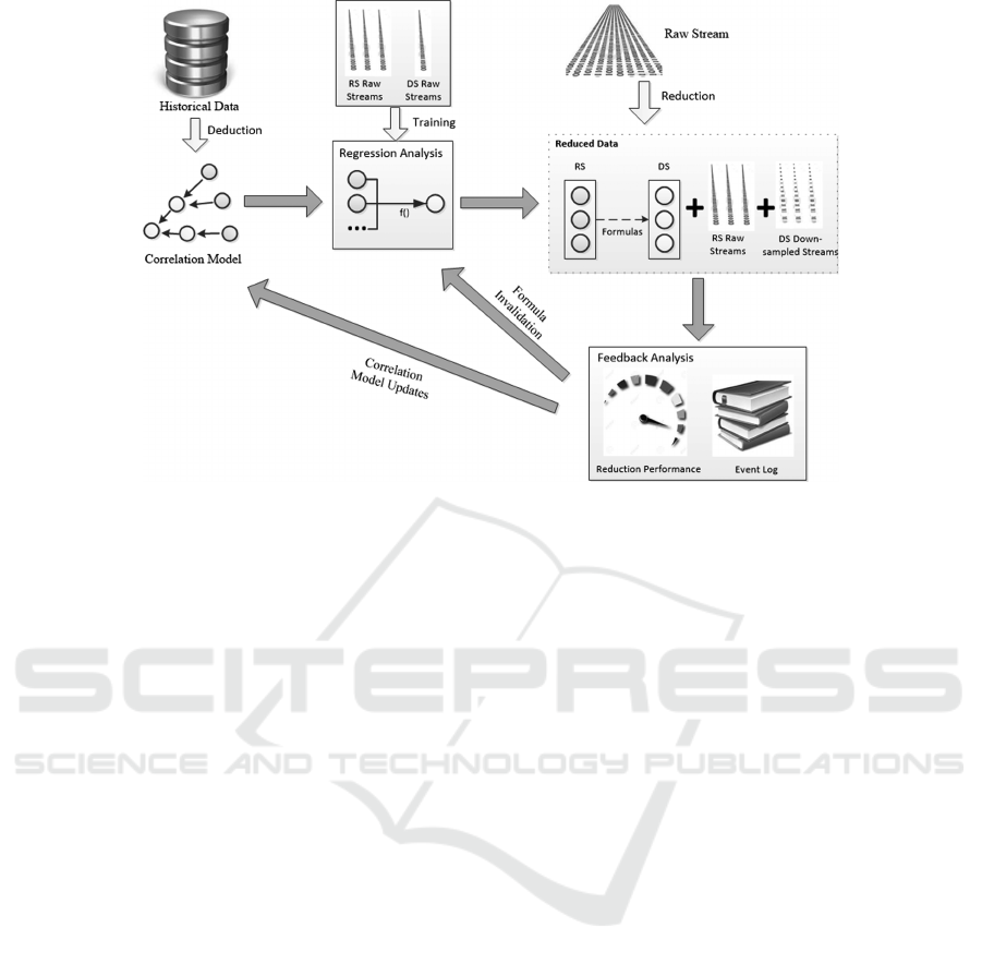
Figure 2: CMBDR prediction framework.
layer and treatment layer, but this paper only intro-
duces the goal layer as depicted in Figure 1, because
it indicates the knowledge of data correlations. In-
stead of using a human expertise, the indicators net-
work automatically learns from historical data. First,
possible relations between indicators are learned by
putting a threshold over their Pearson correlation co-
efficients; then a MMHC-like algorithm (Tsamardi-
nos et al., 2006) is applied to orient all network edges;
finally a Bayesian Network is derived from monitored
data, depicting relations among indicators. Thus, as
the starting point of this paper, this Bayesian Network
model (a DAG) provides correlations between indica-
tors learned from historical data and it gives an initial
input to the data reduction.This paper only takes ad-
vantage of the DAG to serve as a model illustrating
correlations, called correlation model, and a directed
edge from indicator A to indicator B in the model im-
plies that values of B are conditionally dependent on
A, thus we could make predictions of B based on the
value of A.
3.2 CMBDR Framework
Data centers monitor a variety of variables continu-
ously, so values of each variable are in time-series,
among which most are numerical values. In this pa-
per, we refer those numerical variables as indicators,
and we consider the reduction problem of multiple in-
dicators streams. Denoting the set of all indicators as
S, this reduction method proposes to use a subset of
S, referred as Regressor Indicators Set (RS), to predict
values of other indicators, denoted as Dependent In-
dicators Set (DS). We try to find a function F to quan-
tify the relation between DS and RS as Equations 1, 2
show, so that data of dependent indicators can be re-
duced. Namely on the micro level, each dependent
indicator di
m
∈ DS requires a formula f to reproduce
itself based on values of several regressor indicators
ri
n
∈ RS, called Correlated Regressor Set (CRS), as
Equations 3, 4 show. This work achieves two goals:
• Identify appropriate RS/DS and CRS, derive accu-
rate prediction formulas for dependent indicators;
• Reduce data volume of dependent indicators in
data collection.
DS = S − RS (1)
DS = F(RS) (2)
di
m
= f (ri
1
,ri
2
,·· · , r i
l
) (3)
CRS[di
m
] = {ri
1
,ri
2
,·· · , r i
l
} (4)
With known correlations provided by the corre-
lation model and RS/DS configuration, CMBDR re-
curses correlations in the DAG to identify CRS, and
performs regression analyses on values of correlated
indicators in a short period (called training window),
to find a formula fitting the quantitative relations of
these variables. Thus values of the dependent indi-
cator di
m
can be reproduced by the formula and cor-
related indicators CRS[di
m
], achieving data reduction.
This framework conducts model-based reduction in
an online manner, which adjusts the correlation model
and the reduction process based on performance feed-
back. Depicted in Figure 2, CMBDR separates reduc-
tion process into several iterations of the following
four main steps.
Correlation-Model-Based Reduction of Monitoring Data in Data Centers
397

• correlation Model Deduction: Derive the indica-
tors correlation model for the data center as Sec-
tion 3.1 illustrated, assign RS/DS and select the
correlated regressor indicators CRS[di
m
] for each
dependent indicators di
m
;
• Regression Formula Learning: Train a formula
for each dependent indicator to quantify their re-
lations with regressor indicators.
• Dependent Indicators Reduction: Reduce sam-
pling rate of dependent indicators, and adopt pre-
dictions of the formulas to replace lost samples.
• Feedback Analysis: Evaluate the performance of
the reduction process, and try to find possible
problems and solutions to improve it.
The correlation model deduction is based on the
indicator relation network illustrated in Section 3.1,
which specifies highly-correlated indicators. We gen-
erate this indicators network under a variable work-
load, in order to find workload independent correla-
tions. We consider the correlations as a consequence
of interconnections of data center modules, for in-
stance, the CPU usage of a virtual machine is always
correlated to the CPU usage of its host. So we ex-
tract the DAG of the relation network as correlation
model, and with help of this model, we can identify
several indicators capable of predicting dependent in-
dicators. Then we assign the nodes of DAG to RS/DS,
and select correlated regressor indicators CRS[di
m
] of
di
m
by algorithm 1. This algorithm selects regressor
indicators ri ∈ RS to predict the dependent indicator
di ∈ DS if ri has a directed path p to di in the DAG,
and no other regressor indicators exist on the path p.
The selection of RS/DS and CRS has obvious impacts
on reduction performance, so in order to minimize the
size of RS, we select root nodes of the DAG as regres-
sor indicators of the first loop, and select other nodes
as dependent indicators. And if the reduction perfor-
mance is poor under current RS/DS configuration, we
update the RS/DS in the following loops according to
feedback analysis results. In addition, the correlation
model is not static in the framework, we need to re-
compute it if some indicators are added or removed in
the monitoring system.
In the regression formula learning step, in order to
quantify relations between indicators, we exploit re-
gression techniques on correlated indicators. A train-
ing window of streaming data is fetched for each
group of indicators as selected in the first step, then
linear regression analysis is carried out, deriving a
prediction formula f that can reproduce values of the
dependent indicator.
Then in the dependent indicators reduction step,
formulas make predictions to replace raw samples of
Algorithm 1: Select regressor set for each dependent indica-
tor di
m
.
Require: RS, DS, DAG(V,E)
Ensure: CRS {the set of correlated regressor indica-
tors of each di
m
}
Function SelectCRS
Stack stack :=
/
0
for ri in RS do
stack.push( neighbors(ri) ) {find neighbors that
are linked by an edge from current node v}
while stack 6=
/
0 do
v := stack.pop;
if v is in DS then
CRS[v].add(ri)
stack.push( neighbors(v) )
else
continue
end if
end while
end for
return CRS
End Function
the dependent indicators partially. As Figure 2 de-
picts, sampling rates of dependent indicators are re-
duced to a lower level, and the lost samples are re-
placed by the formula predictions, which are derived
out of the values of regressor indicators. Further-
more, we compare samples of the dependent indica-
tors to prediction results, providing a glimpse of ac-
curacy performance. Therefore, the final reduced data
is composed of several parts, namely, all raw samples
of regressor indicators, training samples and check-
ing samples of dependent indicators, and formulas pa-
rameters.
Finally, the framework performs feedback analy-
ses, in which reduction performance and the event log
of the data center are analyzed to generate feedbacks,
helping to improve the next loop. Reduction per-
formance is evaluated with combined-criteria, cover-
ing compression ratio, execution time and informa-
tive value. By spotting the indicators and formulas
with poor performance, we identify problems in each
loop iteration, so we can update the corresponding re-
gression formula and correlation model to improve
performance. In addition, events in the log can also
guide reduction process to adapt to the changes of the
data center environment. For instance, in the feed-
back analysis, if we found a virtual machine is added
to or removed from a host server in feedback analysis,
then we need to recompute the correlation model be-
fore running the next loop. Details will be discussed
in Section 5.
SMARTGREENS 2016 - 5th International Conference on Smart Cities and Green ICT Systems
398
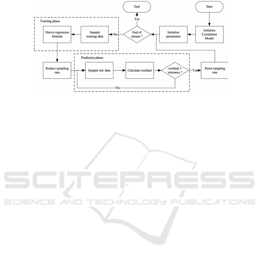
Figure 3: Predictor workflow.
3.3 Indicators Stream Predictor
This section explains the design of the indicators
stream predictor in detail, which is a first implemen-
tation of the CMBDR framework. Based on the cor-
relation model, the predictor tries to figure out for-
mulas of indicators by regression analysis on train-
ing dataset, and reduces their sampling rate to a low
level to serve as check items. Its working procedures
mainly include two phases: training phase and predic-
tion phase, the predictor always trains the formulas in
training phase, and then verifies the formulas in pre-
diction phase. If a prediction result does not match the
sample result, then a prediction failure is generated as
feedback and the corresponding formula needs to be
recomputed in the next training phase. The predic-
tor workflow is depicted in Figure 3. Before predic-
tor running, the correlation model is initialized and
some parameters are configured. Afterwards train-
ing phase starts, predictor carries out regression anal-
ysis for each formula which involves the dependent
indicator di
m
and also correlated regressor indicators
ri ∈ CRS[di
m
]. Subsequently, we cut down sampling
rate of dependent indicators in the prediction phase.
Then we compare each sample with prediction re-
sults, and if their difference (residual) exceeds prede-
fined tolerance, the prediction will be considered as a
failure and the prediction phase of this formula will be
terminated. Finally, a new training phase starts unless
the predictor has reached the end of the stream. In
order to control efficiency and accuracy of the reduc-
tion process, we introduce three important parameters
to the predictor:
• Length of Training Data Set: the number of sam-
ples required to train a formula, denoted as LT;
• Prediction Tolerance: the range for prediction er-
rors (or residuals) within which the prediction will
not be considered as a failure, denoted as PT ;
• Prediction Sampling Rate: sampling rate for de-
pendent indicators in prediction phase, denoted as
SR, which should be generally smaller than the
original sampling rate.
3.4 Linear Regression Method
To achieve our goal, the adopted reduction methods
should have the competence to derive quickly the
quantitative relationship between indicators in a time
slot, and to predict future values of some indicators.
In this approach, we explore methods of regression
analysis to discover formulas quantifying the relation-
ships and predicting values of dependent indicators
based on regressor indicators. Considering the time
to find fitting regression models of streaming indica-
tors, the computation complexity of regression anal-
ysis must be limited. Thus, CMBDR should give
preference to the regression model with the least time
complexity, namely, the linear regression model.
Generally, linear regression is an approach mod-
eling linear formulas between scalar dependent vari-
ables and independent variables. While multiple lin-
ear regression attempts to model the relationship be-
tween two or more independent variables and a re-
sponse variable by fitting a linear equation to ob-
served data (see Equation 5), simple linear regression
is a special case of multiple linear regression having
only one independent variable (see Equation 6). In
the two equations, suppose data consists of n obser-
vations {y
i
,x
i1
, ··· ,x
ip
}
n
i=1
, then x
i j
means the j
th
in-
dependent variable measured for the i
th
observation,
y
i
means the response variable measured for the i
th
observation, α is called intercept, β
j
are called slopes
or coefficients, ε
i
are an unobserved random variable
that adds noise to the linear relationship.
Correlation-Model-Based Reduction of Monitoring Data in Data Centers
399
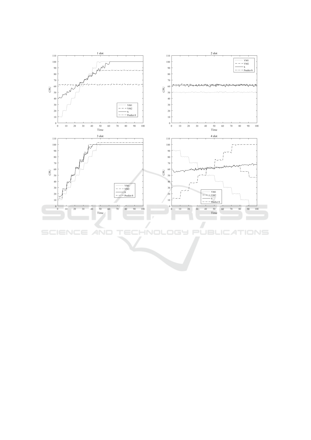
Figure 4: CPU ratios in four patterns (VM
1
- dotted lines, V M
2
- dashed lines, S - solid lines, Prediction of S - dash-dot lines).
y
i
= α + β
1
x
i1
+ ·· · + β
p
x
ip
+ ε
i
(5)
y
i
= α + β
1
x
i
+ ε
i
(6)
If X (the matrix of x
i j
) is full column rank,
CMBDR uses OLS (Ordinary Least Squares) regres-
sion method to estimate parameters of the formula
minimizing SSR (sum of squared residuals) over all
possible values of the intercept and slopes, as shown
in Equation 7. Details of OLS method can be found
in (Hayashi, 2000). If X is not full column rank, then
some column vectors must be linearly dependent, thus
CMBDR applies Gaussian Elimination to get the full
column rank matrix and then applies the OLS method.
SSR =
∑
i
(y
i
− α − β
1
x
i1
− ·· · − β
p
x
ip
)
2
(7)
4 PREDICTION FORMULA
VALIDATION
Regression analysis derives the prediction formula
that best fits training datasets. Therefore, this for-
mula could maintain a high prediction rate on follow-
ing testing data until the quantitative relation changes
and prediction rate dramatically decreases. So under-
standing when the relation will change is quite im-
portant for predictor performance. In this section, in
order to get insights into behaviors of the predictor,
we study prediction failures of the regression formu-
las under certain controlled conditions, by designing
several particular patterns to model typical situations
in data centers and validating prediction formulas in
each situation.
Experiments are conducted in MATLAB with a
data center simulation framework (Vitali et al., 2013).
With proper settings of the simulated data center, we
are able to control the framework to generate monitor-
ing data under specific workload, thus we can evaluate
performance of the predictor on various conditions.
We prepare a simple data center environment with
2 virtual machines (VM) deployed on 1 host server
(S), and CPU usages of VMs are and S are all 3 indi-
cators, in which CPU(V M
1
) and CPU(V M
2
) are re-
gressor indicators and CPU (S) is dependent indicator.
Furthermore, 4 slots of monitoring data are generated
under different workload patterns of VMs, as Fig-
ure 4 illustrates, to simulate possible workload con-
ditions of the data center. In the first slot, workload
of V M
1
increases while V M
2
remains the same, but
SMARTGREENS 2016 - 5th International Conference on Smart Cities and Green ICT Systems
400

Table 1: Indicators configurations in the first loop.
Indicator Description Unit Indicator set Regressor Indicators
CPU(V M
i j
) CPU ratio of j
th
VM deployed on S
i
RS
R(V M
i j
) Response time of j
th
VM deployed
on S
i
ms DS CPU(V M
i j
)
P(V M
i j
) Instant power consumption of j
th
VM deployed on S
i
watt DS CPU(V M
i j
)
CPU(S
i
) CPU ratio of S
i
DS CPU(V M
i1
)··· CPU(V M
i6
)
P(S
i
) Instant power consumption of S
i
watt DS CPU(V M
i1
)···CPU(V M
i6
)
Figure 5: Prediction results in four patterns.
due to the resource limits, the indicators CPU(V M
1
)
and CPU(S) stop increasing when CPU ratios reach
100%, which means the workload requests have ex-
ceeded the processing power. In the second slot, two
VMs workloads remain unchanged, so all indicators
remain stable. In the third slot, both VMs increase
their workloads at almost same speed; in the last slot,
V M
1
increases workload while V M
2
decreases, and
the CPU usage of the host CPU(S) grows slowly.
Each slot consists of 100 samples, and the start-
ing 20 samples are used to train a prediction formula,
which will be tested by all samples left. Applying the
threshold (Prediction Tolerance) to the residual be-
tween sample and prediction, a boolean result is gen-
erated, as Figure 5 depicts. In the beginning, all pre-
diction formulas perform well since most predictions
are accurate. Nevertheless, in pattern 1, 3, 4, the pre-
diction accuracy decreases suddenly afterwards and
it reveals a significant change of indicators relation.
This happens when CPU ratio of a VM reach 100%
so it has to stop the previous trend.
These sudden relation changes can be explained
by overload conditions of VMs and the server. When
a VM get overloaded, the real CPU consumption of
the VM is still increasing even if monitored indica-
tor C PU(V M) remains at 100%, because VM can ac-
quire additional resource from the host server. Thus,
the previous prediction formula cannot explain cur-
Correlation-Model-Based Reduction of Monitoring Data in Data Centers
401

rent overload situations, for instance, from the mid-
dle part of the first slot, the prediction remains stable
since CPU(V M
1
) and CPU(V M
2
) remain unchanged,
but the indicator CPU (S) is still increasing because
the real workload request of V M
1
does not stop in-
creasing.
This experiment demonstrates two outcomes.
First and most importantly, the regression formula of
correlated indicators is capable of making accurate
predictions in certain conditions. Secondly, the quan-
titative relations between indicators are not static, and
they evolve with dynamic data center environment.
Considering these two outcomes, in CMBDR frame-
work, we exploit regression formula to capture tem-
porary quantitative relation between correlated indi-
cators, and model feedback loops to adapt to dynamic
changes of formulas and correlations.
5 EXPERIMENTAL STUDY
In this section, we discuss experimental results
of the described approach to assess the performance
of CMBDR framework. We conduct experiments in
the same simulation tool of data center, which cre-
ates a virtualized data center environment and allows
the collection of simulation data at different work-
load rates. This tool emulates VMs resource alloca-
tion on servers and generates monitoring data such as
resource usage and power consumption under certain
workload rates. It also estimate power consumption
of a VM based on the amount of CPU it consumes.
5.1 Experiment Setting
To reveal the performance of CMBDR predictor, we
test it in a larger data center. This data center consists
of 100 servers with 6 VMs deployed on each server.
Monitoring data stream includes 2000 indicators that
cover CPU usage, response time and power consump-
tion of both VMs and servers. As Table 1 depicts, in
the initial reduction loop of CMBDR framework, we
select root nodes (namely, CPU(VM
i j
)) of the corre-
lation model as regressor indicators, and take other
nodes as dependent indicators. Testing data are gen-
erated by the simulation tool under simulated daily
workloads, with sampling rate of 1 per minute (1440
samples in one day).
As an important parameter of the predictor, pre-
diction tolerance PT defines the threshold for pre-
diction errors and has a great influence on reduction
results. In this work, the value of PT is directly
based on the measurement error of raw monitoring
data. We first put the data center in a stable work-
load conditions, and collect values of indicators for a
period. Therefore, the multiple samples are repeated
measurements on the same state of the data center,
they should follow normal distribution around the true
value µ and variance is σ
2
, as Equation 8 depicts.
Therefore, we exploit the 95% confidence interval
(approximately 1.96×σ) as a criteria for error behav-
ior of raw samples, and assign it to PT as Equation 9
shows. We consider the raw sample and the corre-
sponding prediction as two observations on the same
indicator, and if the difference between these two ob-
servations is within the 95% confidence interval, this
prediction could be viewed as an accurate measure-
ment, namely, a true prediction.
measurement ∼ N(µ,σ
2
) (8)
PT = 1.96 × σ (9)
5.2 Evaluation Criteria
In order to evaluate the indicator stream predictor
comprehensively, this work proposes combined eval-
uation criteria covering operation speed, reduction
volume and informative values of reduced data. In-
formation value is a general term describing the abil-
ity of reduced data for supporting target applications;
it could be distinct for wide varieties of applications.
Thus, we exploit multiple metrics instead of a single
criterion to measure informative values. Details of the
combined evaluation metrics are as follows.
• Execution Time: processing time for the predictor
to reduce prepared data stream.
• Reduction Volume: the difference between raw
data size and reduced data size.
• Hit Rate: Consider the prediction within the error
range of raw data as a hit, thus the hit rate is the
percentage of accurate predictions, which reflects
informative values of reduced data.
• Relative Error: this metric measures information
loss of data reduction process, as shown in equa-
tion 10, for each indicator, η is relative error, ε is
absolute error and v is the interval of the values in
the test dataset.
η =
ε
v
(10)
• Weighted mean of R
2
: R
2
is often used to measure
total goodness of fit of linear regression models,
as equation 11 depicts, y
i
is raw value and f
i
is
prediction value. and R
2
= 1 indicates that the re-
gression line perfectly fits raw data. In this work,
R
2
is used to measure accuracy in each predic-
tion phase, and length-based weighted average of
SMARTGREENS 2016 - 5th International Conference on Smart Cities and Green ICT Systems
402

Table 2: Prediction performance of formulas in the same category.
R(V M) P(V M) CPU(S) P(S) P(S)revision
Relative error 3.45E-03 1.97E-03 4.82E-02 4.86E-02 1.19E-04
Average R
2
0.889 0.917 0.220 0.208 1.000
Hit rate 95.96% 98.57% 82.01% 81.85% 100.00%
Reduction volume 1241.46 1304.32 900.37 893.20 1339.25
Execution time sec. 0.144 s 0.070 s 0.680 s 0.690 s 0.029 s
those R
2
on data stream will be used as a metric
to evaluate how well predictions fit raw data.
R
2
= 1 −
∑
n
i=1
(y
i
− f
i
)
2
∑
n
i=1
(y
i
− y)
2
(11)
5.3 Formulas Revisions
In the experiment, we monitor the reduction process,
and measure performance of each formula using the
aforementioned criteria. One interesting point we
found is that the variability of prediction ability is sig-
nificant between formulas. Some formulas can make
very accurate predictions in a short execution time
while some formulas fail frequently and cost more
time to train new formulas. The reason for this dis-
crepancy lies in the correlation model. In the reduc-
tion process, if a prediction formula does not meet ac-
curacy requirements, then the predictor needs to learn
a new regression formula to replace t, thus the for-
mula could be always up-to-date. However, some de-
pendent indicators may be hard to predict by selected
regressor indicators, if their correlations are not high
enough. Thus, the framework would take much time
to update those formulas frequently, even though the
general performance increases very little.
Therefore, in order to solve the problem, the pre-
dictor need to revise those inefficient formulas in the
next reduction loop. We denote dependent indicators
of those foot-dragging formulas as slowDS, and we
need to expand RS to include a subset of slowDS to
enhance prediction ability, since results have proved
current RS is not capable of making accurate predic-
tions on those indicators. Among all possible solu-
tions, adding the complete set of slowDS to RS can
solve the issue all at once, but obviously it can only
achieve minimal data reduction. This work recon-
siders correlations between indicators of slowDS in
the correlation model, it obtains several disconnected
subgraphs of the DAG containing only the slowDS
nodes, and add the root nodes of subgraphs to RS.
For instance, if any indicators of slowDS are corre-
lated, they must exist in the same subgraph, thus the
corresponding root node would serve as the regressor
indicator for other nodes in the next loop; otherwise
all slowDS will serve as regressor indicators. By this
gradual means of expanding RS, appropriate RS/DS
could be identified in iterations of reduction loops.
In this experiment, CMBDR framework selects
the root nodes of correlation model as RS in the first
loop. Individual performance of indicators in the first
loop are evaluated in the first 4 columns of Table 2,
each column representing the average performance
of indicators in the same category. Under initial
RS/DS configuration, the indicators of R(V M
i j
) and
P(V M
i j
) outperform evidently CPU (S
i
) and P(S
i
),
with higher reduction volume, better prediction ac-
curacy and much less execution time. To acquire
better performance in the second loop iteration, we
need to update RS/DS. By querying in the correlation
model, we find CPU(S
i
) and P(S
i
) are highly corre-
lated. Then we just move one indicator CPU(S
i
) from
DS to RS, and then call Algorithm 1 to update regres-
sor set CRS for P(S
i
), thus CPU(S
i
) would be used to
predict P(S
i
) in the second loop. The performance are
also measured, as the fifth column in Table 2 shows,
both accuracy and execution speed are improved dra-
matically and the relative error is at the same level
with P(V M
i j
).
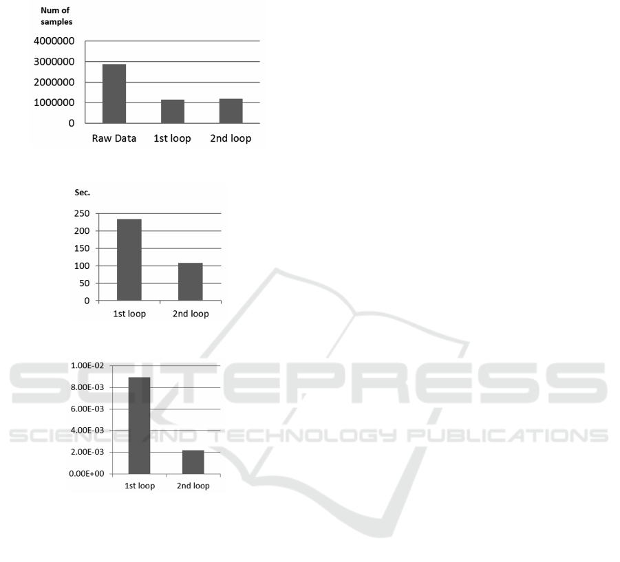
We also measure overall reduction performance
of monitoring data in reduction process, to verify the
validity of this predictor and to assess the improve-
ment offered by RS/DS updates. As Figure 6 depicts,
in both first and second loops, the predictor reduces
the raw monitoring data to slightly above one-third of
original volume, and reduction of 2 loops are nearly
the same although the predictor involves more regres-
sor indicators in the second loop. However, these new
regressor indicators improve processing speed and ac-
curacy performance of the predictor dramatically. As
Figure 7 and Figure 8 show, the second loop doubles
processing speed of the first loop, and increases aver-
age prediction accuracy by almost an order of mag-
nitude. Results of the second loop in Figures 7, 8
also illustrate that, for a data center of 2000 indica-
tors, this predictor is able to reduce daily monitoring
data within 100 seconds, ensuring the average relative
error at 10
−3
.
Above all, this predictor could cut down the vol-
ume of data collection in monitoring systems, while
Correlation-Model-Based Reduction of Monitoring Data in Data Centers
403
still maintaining fast speed and a good quality of in-
formative values.
Figure 6: Data volume before and after reduction.
Figure 7: Execution time of CMBDR loops.
Figure 8: Average relative error of the predictor.
6 CONCLUSIONS
In this work, we developed and implemented a data
reduction framework for a data center monitoring sys-
tem. We derived the correlation model of indicators,
and based on correlations, we built a stream predictor
to decrease sampling of raw data by deducing quan-
titative relations between indicators. We have also
designed the feedback loop in the reduction process,
which evaluates and optimizes reduction performance
in iterations, enhancing adaptability of the correlation
model and formulas in a dynamic environment. Vali-
dation results show that regression formulas can pre-
dict indicators under typical workload patterns, and
predictor test results demonstrate that this approach
is capable of reduction in a simulated data center.
This mechanism could provide an extension to other
solutions in terms of upstream data reduction, and
it serves as a practical solution for monitoring data
streams in which variables are commonly correlated.
Future work may be carried on data center anomaly
detection, or fault-tolerant mechanisms of monitoring
data, which also exploits data correlations to establish
standby channels in monitoring systems, as in (Zhou
et al., 2015).
ACKNOWLEDGEMENTS
This work has been partially funded by the Italian
Project ITS Italy 2020 under the Technological Na-
tional Clusters program.
REFERENCES
Carvalho, C., Gomes, D. G., Agoulmine, N., and De Souza,
J. N. (2011). Improving prediction accuracy for
wsn data reduction by applying multivariate spatio-
temporal correlation. Sensors, 11(11):10010–10037.
Ding, R., Wang, Q., Dang, Y., Fu, Q., Zhang, H., and
Zhang, D. (2015). Yading: fast clustering of large-
scale time series data. Proceedings of the VLDB En-
dowment, 8(5):473–484.
Esling, P. and Agon, C. (2012). Time-series data mining.
ACM Computing Surveys (CSUR), 45(1):12.
Hayashi, F. (2000). Econometrics. Princeton Univ. Press,
Princeton, NJ [u.a.].
Jolliffe, I. (2002). Principal component analysis. Wiley
Online Library.
Keogh, E., Chakrabarti, K., Pazzani, M., and Mehrotra, S.
(2001). Dimensionality reduction for fast similarity
search in large time series databases. Knowledge and
information Systems, 3(3):263–286.
Kung, H., Lin, C.-K., and Vlah, D. (2011). Cloudsense:
Continuous fine-grain cloud monitoring with com-
pressive sensing. In HotCloud.
Peng, X. (2015). Data reduction in monitored data. In
Loucopoulos, P., Nurcan, S., and Weigand, H., editors,
Proceedings of the CAiSE’2015 Doctoral Consortium
at the 27th International Conference on Advanced In-
formation Systems Engineering (CAiSE 2015), Stock-
holm, Sweden, June 11-12, 2015., volume 1415 of
CEUR Workshop Proceedings, pages 39–46. CEUR-
WS.org.
Reeves, G., Liu, J., Nath, S., and Zhao, F. (2009). Manag-
ing massive time series streams with multi-scale com-
pressed trickles. Proceedings of the VLDB Endow-
ment, 2(1):97–108.
Tsamardinos, I., Brown, L. E., and Aliferis, C. F. (2006).
The max-min hill-climbing bayesian network struc-
ture learning algorithm. Machine learning, 65(1):31–
78.
SMARTGREENS 2016 - 5th International Conference on Smart Cities and Green ICT Systems
404

Vitali, M., O’Reilly, U.-M., and Veeramachaneni, K.
(2013). Modeling service execution on data centers
for energy efficiency and quality of service monitor-
ing. In Systems, Man, and Cybernetics (SMC), 2013
IEEE International Conference on, pages 103–108.
IEEE.
Vitali, M., Pernici, B., and OReilly, U.-M. (2015). Learn-
ing a goal-oriented model for energy efficient adap-
tive applications in data centers. Information Sciences,
319:152–170.
Zhou, S., Lin, K.-J., Na, J., Chuang, C.-C., and Shih, C.-S.
(2015). Supporting service adaptation in fault toler-
ant internet of things. In Service-Oriented Comput-
ing and Applications (SOCA), 2015 IEEE 8th Inter-
national Conference on, pages 65–72.
Correlation-Model-Based Reduction of Monitoring Data in Data Centers
405
