Dynamic Pricing and Energy Management Strategy for EV Charging
Stations under Uncertainties
Chao Luo, Yih-Fang Huang and Vijay Gupta
Department of Electrical Engineering, University of Notre Dame, Notre Dame, Indiana, U.S.A.
Keywords:
Electric Vehicle, Charging Station, Dynamic Pricing, Energy Management, Dynamic Programming,
Renewable Energy Integration.
Abstract:
This paper presents a dynamic pricing and energy management framework for electric vehicle (EV) charging
service providers. To set the charging prices, the service providers faces three uncertainties: the volatility
of wholesale electricity price, intermittent renewable energy generation, and spatial-temporal EV charging
demand. The main objective of our work here is to help charging service providers to improve their total
profits while enhancing customer satisfaction and maintaining power grid stability, taking into account those
uncertainties. We employ a linear regression model to estimate the EV charging demand at each charging
station, and introduce a quantitative measure for customer satisfaction. Both the greedy algorithm and the
dynamic programming (DP) algorithm are employed to derive the optimal charging prices and determine how
much electricity to be purchased from the wholesale market in each planning horizon. Simulation results show
that DP algorithm achieves an increased profit (up to 9%) compared to the greedy algorithm (the benchmark
algorithm) under certain scenarios. Additionally, we observe that the integration of a low-cost energy storage
into the system can not only improve the profit, but also smooth out the charging price fluctuation, protecting
the end customers from the volatile wholesale market.
SYMBOLS
N: total number of planning horizon.
s
j
: the j-th EV charging station.
p
k j
; charging price of the j-th charging station in
the k-th horizon.
c
k
: electricity wholesale price in the k-th horizon.
E: electricity storage capital.
R
k
: total revenue in the k-th horizon.
o
k
: electricity purchase in the k-th horizon.
d
k j
: charging demand at the j-th charging station
in the k-th horizon.
G
k
: overall customer satisfaction.
β: weighting parameter of customer satisfaction.
α: shape parameter for customer satisfaction
function.
ω: shaping parameter for customer satisfaction
function.
φ
k
: total charging demand in the k-th horizon.
Q
k
: stress imposed on power grid due to EV
charging in the k-th horizon.
o
ref
: reference electricity purchase (average
electricity purchase).
o
max
: maximum electricity purchase.
µ: weighting parameter of electricity purchase
fluctuation.
I
k
: electricity storage at the beginning of the k-th
horizon.
u
k
: renewable energy generation in the k-th
horizon.
W
k
: electricity storage cost in the k-th horizon.
η: unit electricity storage cost.
Π
k
: total utility in the k-th horizon.
γ
i, j
: price elasticity parameter.
J
k
(I
k
): maximum aggregated utility from the k-th
horizon to the last horizon.
1 INTRODUCTION
Recent innovations in battery and powertrain tech-
nology have served as a catalyst for expediting
Luo, C., Huang, Y-F. and Gupta, V.
Dynamic Pricing and Energy Management Strategy for EV Charging Stations under Uncertainties.
In Proceedings of the International Conference on Vehicle Technology and Intelligent Transport Systems (VEHITS 2016), pages 49-59
ISBN: 978-989-758-185-4
Copyright
c
 2016 by SCITEPRESS – Science and Technology Publications, Lda. All rights reserved
49

the proliferation of electric vehicles (EVs). EVs
exhibit many advantages over the internal combustion
engine (ICE) vehicles, including lower operation cost,
higher fuel conversion efficiency, and reduced or
eliminated tailpipe emission (Simpson, 2006; IEC,
2007). The American market share of plug-in EVs
in new registered cars increased from 0.14% to
0.37% in 2012, 0.62% in 2013, and 0.72% in 2014
(Electric Drive Transportation Association, 2015).
According to Navigant Research, the global light duty
EV market is expected to grow from 2.7 million
vehicle sales in 2014 to 6.4 million in 2023 (Navigant
Research, 2014). EVs will play a significant role
in transportation electrification. Nevertheless, the
limited driving range and the long charging time are
still the major obstacles to the proliferation of EVs.
The “range anxiety” is like the Sword of Damocles
for EV owners. More charging stations need be
established to alleviate the “range anxiety”. In
addition, the profitability of the EV charging industry
is another critical issue that should be considered.
The EV charging industry needs a promising business
model to bring more private investors into this
industry instead of solely relying on financial support
or incentives from governments. The effective and
efficient management of charging infrastructure is at
the heart of the EV charging industry. The objective
of this paper is to provide guidelines for charging
service providers make informed and optimized
decisions on pricing and energy management so
as to coherently improve profits, enhance customer
satisfaction, and reduce uncertainties or risks.
Currently, there is a plethora of literature aiming at
addressing the dynamic pricing issue of EV charging
stations. Yan et al. proposed a multi-tiered real-
time pricing algorithm for charging stations by taking
into account both the day-ahead predicted electricity
price and the real-time load information (Yan et al.,
2014). However, they did not consider the possibility
that EV owners may change their charging behavior
in response to the varying prices. Han et al.
presented a dynamic pricing and scheduling scheme
for EV charging stations while considering grid-to-
vehicle (G2V) and vehicle-to-grid (V2G) (Han et al.,
2012). They used a Stackelberg game to characterize
the strategic interactions between the “selfish” EV
owners and the charging stations. However, they only
considered a single charging station in their model.
In (Ban et al., 2012), a price control method was
employed to guide EVs to different charging stations
while satisfying the predefined QoS and maintaining
power grid stability. The authors used a multi-queue
system to model the arrival and departure of EVs.
Nevertheless, they treated the charging station as a
profit-neutral entity, which may not be an appropriate
assumption for the real market. In (Martirano et al.,
2014), the authors proposed a scheme called the
“Interactive Energy”, for the dynamic pricing and
electricity delivery of the EV charging services based
on the status of the microgrid. However, the overall
customer satisfaction was not considered in their
analysis. The pricing models proposed in (Rahbari-
Asr et al., 2013) and (Guo et al., 2014) did not
incorporate the renewable energy (like wind power or
solar power), which is becoming an important energy
source. In (Guo et al., 2016), the authors addressed
a two-stage framework for the economic operation of
a microgrid-like electric vehicle parking deck using
a stochastic approach and model predictive control
(MPC).
Our work is motivated by the fact that the
charging service providers face many uncertainties
when determining the appropriate charging prices
and managing the electricity storage. In this paper,
we consider three types of uncertainties that the
service providers may face: (1) the uncertainty of
spatial-temporal charging demand at each charging
station, (2) the uncertainty of renewable energy
generation, and (3) the uncertainty of the electricity
price at the wholesale market. We also assume that
a charging service provider operates a network of
charging stations. As a mediator in the power grid,
the service provider purchases the electricity from
the wholesale market and resells it to EV owners.
We also assume that the service provider owns a
storage system that stores the excessive electricity
temporarily. Additionally, the service provider can
harvest the distributed renewable energy generation,
and use it as a supplementary energy source for EV
charging.
In our study here, we first employ a linear
regression model to estimate the EV charging
demand. Specifically, the customer’s price elasticity
coefficients, reflecting the customer’s sensitivity to
charging price variation, will be estimated using
historical data. Subsequently, we apply the Dynamic
Programming (DP) computation algorithm to derive
the optimal charging prices and how much electricity
to be purchased from the wholesale market based on
the current electricity storage and renewable energy
forecast.
The main contribution of this paper is a
computation framework to help the EV charging
service provider calculate the optimal charging prices
and determine the appropriate amount of electricity to
purchase from the wholesale market in each planning
horizon. Our computation framework can deal with
the three aforementioned uncertainties and is aimed
VEHITS 2016 - International Conference on Vehicle Technology and Intelligent Transport Systems
50

at striking a balance among the profit, customer
satisfaction, and the power grid stability.
2 PROBLEM FORMULATION
In our model, we postulate that there is an EV
charging service provider operating a network of
charging stations. As a mediator between the power
grid and the end customers (i.e., EV owners), the
charging service provider purchases electricity from
the wholesale market at the day-ahead prices, and
resells it to EV owners at the retail charging price.
Figure 1 depicts a general business model for EV
charging.
Electric vehicles
Power plants Charging service provider
Renewable energy
MWh
kWh
Wholesale
Retail
Figure 1: The EV Charging Market.
2.1 Profit of The Service Provider
The worldwide deregulation of electricity market
(e.g., PJM Interconnection, ERCOT in USA, New
Zealand, Singapore, UK markets, etc.) gives
birth to the prosperous forward markets and day-
ahead markets. The Independent System Operator
(ISO) or the Regional Transmission Organization
(RTO) calculates the day-ahead market prices through
an auction between the power generators and the
retailers using the locational marginal pricing (LMP)
scheme (Huisman et al., 2007; Treinen, 2005; Frame,
2001). We assume that the charging service provider
is one of the retailers, buying electricity from the
wholesale market and reselling it to EV owners.
Let S = [s
1
,s
2
,··· ,s
L
] denote the set of charging
stations. We divide a day into N planning horizons
(stages). At the beginning of each horizon, the service
provider updates the charging prices, and calculates
how much electricity needs to be purchased from
the wholesale market. We allow charging prices
vary among different charging stations. Let P
k
=
[p
k1
, p
k2
,··· , p
kL
](k = 1, 2,· ·· ,N) be the charging
price vector in the k-th horizon, and o
k
be the
electricity purchase. Currently, the day-ahead market
prices are calculated on a hourly basis, so N = 24. Let
C = [c
1
,c
2
,··· ,c
N
] denote the day-ahead wholesale
market prices. The total profit of the service provider
in the k-th horizon is given by
R
k
=
L
∑
j=1
p
k j
d
k j
− c
k
o
k
(k = 1,2, ·· · ,N), (1)
where d
k j
is the charging demand at the j-th charging
station in the k-th horizon, and
∑
L
j=1
p
k j
d
k j
is the total
revenue, and c
k
o
k
is the cost of electricity purchased
in the k-th horizon.
2.2 Customer Satisfaction Evaluation
The charging service provider attempts to achieve
the goals of improving the profits, enhancing the
customer satisfaction, and maintaining power grid
stability. Poor customer satisfaction may hinder
the wide adoption of EVs, thus, affecting the
development of the entire EV industry. In this sense,
the charging service provider cannot be a myopic
profit squeezer that maximizes the profit at the
expense of customer satisfaction. Various customer
satisfaction evaluation methods have been studied in
(Yang et al., 2013; Fahrioglu et al., 1999; Faranda
et al., 2007). In this paper, we use a quadratic function
to characterize the overall customer satisfaction of the
entire population of EV owners, denoted by G
k
.
G
k
= β

ωφ
k
−
α
2
φ
2
k

, 0 ≤ φ
k
≤ E (2)
where β is the weighting parameter and E is the
capacity of the electricity storage system, ω and α
are the shape parameters of this quadratic function.
The variable φ
k
is the total electricity consumption
(charging demand) of all EV owners in the k-th
horizon which is defined as
φ
k
=
L
∑
j=1
d
k j
. (3)
The quadratic functions with different combina-
tions of ω and α are shown in Figure 2. We observe
that the quadratic function has a minimum value of
0, suggesting that the EV owners are very “unhappy”,
and a maximum value of 1, suggesting that the EV
owners are very “happy”. Additionally, Equation
(2) is a non-decreasing concave function with a non-
increasing first-order derivative. The overall customer
satisfaction grows as the total electricity consumption
increases. However, the decreasing growth rate
suggests that the customer satisfaction tends to get
saturated as the electricity consumption increases.
Dynamic Pricing and Energy Management Strategy for EV Charging Stations under Uncertainties
51

0 20 40 60 80 100 120 140 160 180 200
0
0.1
0.2
0.3
0.4
0.5
0.6
0.7
0.8
0.9
1
φ
k
(MWh)
Customer satisfaction
ω=0.01,α=0.00005
ω=0.0075,α=0.000025
ω=0.0067,α=0.0000167
Figure 2: Customer Satisfaction Functions (E = 200).
2.3 Impact of EV Charging on Power
Grid
Many studies (Lopes et al., 2011; Kinter-Meyer et al.,
2007; Scott et al., 2007) have shown that large-scale
simultaneous EV charging presents many challenges
to the existing power grid pertaining to severe power
loss, power grid stability, frequency drift, and voltage
fluctuation, etc. In the electric power system,
the networked generators cooperatively adjust their
outputs to balance the supply and the demand and
maintain the power quality. Generally, the power
generators hope that the load is predictable and
relatively stable (or at least slow-varying). If the
load fluctuates too much, the power generators have
to ramp up and down frequently, resulting in low
efficiency and high maintenance cost. As a result,
we do not want the electricity purchase from the
wholesale market o
k
to fluctuate too much which
may create a heavy “burden” on the power grid. We
formulate the penalty of EV charging in the following
way
Q
k
= µ(o
k
− o
ref
)
2
, (4)
where o
ref
is a reference purchase (or average
electricity purchase) and o
k
is the electricity
purchased in the k-th horizon. The variable µ is
the weighting parameter reflecting the sensitivity of
electricity purchase fluctuation.
2.4 Cost of Electricity Storage
We assume that the charging service provider has an
electricity storage with a capacity of E(MWh). Let I
k
denote the electricity in the storage at the beginning of
the k-th horizon, and let u
k
be the renewable energy
generation (i.e. wind power or solar power). Here
u
k
is the predicted renewable energy. The electricity
storage cost in the k-th horizon is given as follows
W
k
= η(I
k
+ u
k
+ o
k
−
L
∑
j=1
d
k j
), (5)
where
∑
L
j=1
d
k j
is the total charging demand in the k-
th horizon, and η($/MWh) is the unit storage cost.
The storage cost includes capital cost, maintenance
cost, and power loss due to energy conversion.
Finally, the total utility of the service provider in
the k-th horizon is given as
Π
k
= R
k
+ G
k
− Q
k
−W
k
=
L
∑
j=1
p
k j
d
k j
− c
k
o
k
+ β

ωφ
k
−
α
2
φ
2
k

−
µ(o
k
− o
ref
)
2
− η(I
k
+ u
k
+ o
k
−
L
∑
j=1
d
k j
),
(6)
Note that the total utility consists of four
components—total revenue, customer satisfaction,
power grid influence, and electricity storage cost. The
values of β and µ reflect the weights of customer
satisfaction and EV charging penalty in the total
utility function.
Our objective here is to maximize the overall
utility by solving the following optimization problem.
(P
∗
1
,o
∗
1
,··· ,P
∗
N
,o
∗
N
) = argmax
P
1
,o
1
,···,P
N
,o
N
(
N
∑
k=1
Π
k
)
,
s.t.













0 ≤ o
k
≤ o
max
;k = 1,2,··· , N
p
k j
≥ 0; j = 1,2, ·· · ,L
I
k
+ o
k
−
∑
L
j=1
d
k j
≥ 0
I
k
+ o
k
−
∑
L
j=1
d
k j
≤ E
d
k j
≥ 0; j = 1,2, ·· · ,L
(7)
where P
k
and o
k
are , respectively, the charging price
vector and electricity purchase in the k-th horizon.
To resolve this problem, we are facing two major
challenges: (1) accurately estimate the charging
demand φ
k
, and (2) solve the large-scale optimization
problem in a more efficient way. In the following
sections, we will discuss these problems in more
details.
3 SPATIAL-TEMPORAL
CHARGING DEMAND
ESTIMATION
In this section, we consider the estimation of the
charging demand φ
k
. The charging demand function
VEHITS 2016 - International Conference on Vehicle Technology and Intelligent Transport Systems
52

characterizes the customer’s responsiveness to the
fluctuation of charging prices, for EV owners may
adjust their charging demand or schedule in response
to the variation of charging prices.
In the initial phase of the optimization framework,
we do not have the information of the EV owner’s
responsiveness to the charging prices. We thus apply
a linear regression model to learn and predict the
charging demand φ
k
. For each charging station j( j =
1,2,··· , L), the charging demand is expressed by











d
k1
= γ
0,1
− γ
1,1
p
k1
+ γ
2,1
p
k2
+ ··· +γ
N,1
p
kN
+ ε
k1
,
d
k2
= γ
0,2
+ γ
1,2
p
k1
− γ
2,2
p
k2
+ ··· +γ
N,2
p
kN
+ ε
k2
,
.
.
.
d
kL
= γ
0,L
+ γ
1,L
p
k1
+ γ
2,2
p
k2
+ ··· −γ
N,L
p
kN
+ ε
kL
,
(8)
where γ
0, j
( j = 1, 2,· ·· ,L) is the intercept of the j-th
linear regression equation, and γ
i, j
= γ
j,i
(i 6= j) are the
cross-price elasticity parameters, reflecting how the
change of the charging price of station j can influence
the charging demand at station i. And γ
i,i
is the self-
price elasticity parameter, reflecting how the change
of the charging price of station i can influence its own
charging demand.
In this work, we employ the recursive least
square (RLS) (Proakis, 2007) method to estimate the
elasticity demand parameters from historical data. Let
W
j
= [γ
0, j
,γ
1, j
,··· ,γ
N, j
] denote the price elasticity
parameter vector relevant to charging station j( j =
1,2,··· , L). Applying the RLS algorithm, we have
the following update formula











e
k j
= d
k j
− P
T
k
W
j
,
g
k j
=
H
(k−1) j
P
k
λ+P
T
k
H
(k−1) j
P
k
,
H
k j
= λ
−1
H
(k−1) j
− g
k j
P
T
k
λ
−1
P
k
,
W
j
← W
j
+ e
k j
g
k j
,
(9)
where e
k j
is the prediction error and λ is the forgetting
factor. In initialization, H
0 j
is the identity matrix and
P
0
is an all-zero vector.
Note that Equation (8) captures both the spatial
and temporal fluctuation of charging demand. The
difference in population density, traffic flow, and
urbanization level may result in the spatial fluctuation
of charging demand. Thus, we use different linear
regression equations to estimate different charging
stations. On the other hand, the use of RLS algorithm
enables us to characterize the temporal fluctuation of
charging demand. It keeps track of the most recent
changes in customer’s charging behavior because the
price elasticity parameters will be updated once a new
data is observed.
4 PRICING POLICIES: GREEDY
ALGORITHM VS DP
ALGORITHM
Note that Equation (7) is a complex optimization
problem with N(L+1) decision variables and N(2L +
3) constraints. It is mathematically cumbersome
and hardly feasible to solve this problem in a
brute force manner. One approach is to divide the
original optimization problem into N independent
subproblems. Each horizon corresponds to a
subproblem, and then employ the greedy search
algorithm. This idea will be further discussed in
Subsection 4.1.
On the other hand, we observe that the original
problem exhibits the properties of overlapping
subproblems and optimal substructure, which can
be exploited to solve this problem more efficiently.
Here, we apply the dynamic programming (DP)
computation algorithm to the original problem. DP
is a computation algorithm of solving a large-scale
complex problem by partitioning it into a set of
smaller and simpler subproblems (Cormen et al.,
2001; Bertsekas, 2000). By solving and combining
these subproblems in a forward (bottom-up) or
backward (top-down) fashion, we can obtain the
solution to the original problem. In contrast to the
brute force approach, DP can significantly accelerate
computation speed and save storage. We will discuss
DP in Subsection 4.2.
4.1 Greedy Algorithm
The original optimization problem in Equation (7)
aims to maximize the total utility over N horizons.
The control variables are “chained” in the sense that
the decision variables in the previous horizon can
influence the decision variables in the current horizon.
For simplicity, we ignore the correlation between
adjacent horizons, and try to maximize the utility in
each individual horizon. Specifically, we attempt to
solve the following problem in the k-th horizon,
(P
∗
k
,o
∗
k
) = argmax
P
k
,o
k
{
Π
k
}
s.t.













0 ≤ o
k
≤ o
max
;k = 1,2,··· , N
p
k j
≥ 0; j = 1,2, ·· · ,L
I
k
+ o
k
−
∑
L
j=1
d
k j
≥ 0
I
k
+ o
k
−
∑
L
j=1
d
k j
≤ E
d
k j
≥ 0; j = 1,2, ·· · ,L
(10)
where P
k
and o
k
are , respectively, the charging price
vector and electricity purchase in the k-th horizon. We
Dynamic Pricing and Energy Management Strategy for EV Charging Stations under Uncertainties
53

will use the greedy algorithm as a benchmark in the
simulations.
4.2 Dynamic Programming Algorithm
Note that the hourly-based wholesale electricity
prices are only posted day ahead. We analyse the
dynamic pricing problem with finite horizons (stages)
with N = 24. The system dynamics are expressed by
the evolution of some variables, or the system’s state
variables, under the influence of the decision variables
at the beginning of each horizon (stage) (Bertsekas,
2000; Nemhauser, 1996). The system dynamics are
expressed by the following evolution equation
I
k+1
= I
k
+ u
k
+ o
k
− φ
k
= I
k
+ u
k
+ o
k
−
L
∑
j=1
d
k j
= f (I
k
,u
k
,P
k
,o
k
),k = 1, 2,· ·· , N
(11)
where I
k
is the state variable, representing the
electricity storage at the beginning of the k-th
horizon. The variables u
k
and o
k
are, respectively, the
renewable energy and the electricity to be purchased
from the wholesale market. The charging demand
in the k-th horizon is φ
k
. Note that φ
k
is actually
a function of the charging price vector P
k
, and the
decision variables of the system are (P
k
,o
k
). The
aggregated utility of the service provider from the first
horizon to the Nth horizon is given by
Π
N+1
(I
N+1
) +
N
∑
k=1
Π
k
(I
k
,P
k
,o
k
), (12)
where Π
N+1
(I
N+1
) is the terminal utility incurred at
the end of the process. We can assign a heuristic value
for the terminal utility. The maximum utility J
1
(I
1
) is
given by the following form
J
1
(I
1
) =
max
P
1
,o
1
,···,P
N
,o
N
(
Π
N+1
(I
N+1
) +
N
∑
k=1
Π
k
(I
k
,P
k
,o
k
)
)
,
(13)
Furthermore, the utility J
1
(I
1
) can be calculated in a
recursive manner as follows
J
1
(I
1
) = max
P
1
,o
1
{
Π
1
(I
1
,P
1
,o
1
) + J
2
(I
2
)
}
, (14)
or
J
1
(I
1
) = max
P
1
,o
1
{
Π
1
(I
1
,P
1
,o
1
) + J
2
( f (I
1
,u
1
,P
1
,o
1
))
}
,
(15)
where J
2
(I
2
) is given by
J
2
(I
2
) =
max
P
2
,o
2
,···,P
N
,o
N
(
Π
N+1
(I
N+1
) +
N
∑
k=2
Π
k
(I
k
,P
k
,o
k
)
)
,
(16)
We can apply Equation (15) recursively from the Nth
horizon backward to the first horizon to derive the
solution J
1
(I
1
). The detailed derivation of Equation
(13) to Equation (15) is given in Appendix.
Let X
k
= [p
k1
, p
k2
,··· , p
kL
,o
k
]
T
denote the deci-
sion variables. Moreover, the recursive DP formula
can be rewritten as one of quadratic programming as
follows,
J
k
(I
k
) = max
X
k
∈Z(X
k
)
n
1
2
X
T
k
QX
k
+ B
T
k
X
k
+ r
k
o
, (17)
where Z(X
k
) is the feasible solutions derived from the
constraints in Equation (7). The matrix Q is given by







−2γ
1,1
− αβΓ
2
1
··· 2γ
1,L
− αβΓ
1
Γ
L
0
2γ
2,1
− αβΓ
2
Γ
1
··· 2γ
2,L
− αβΓ
2
Γ
L
0
.
.
.
.
.
.
2γ
L,1
− αβΓ
L
Γ
1
··· −2γ
L,L
− αβΓ
2
L
0
0 ··· 0 −µ







(18)
where Γ
j
( j = 1, 2,· ·· , L) is
Γ
j
= −γ
j, j
+
L
∑
i=1,i6= j
γ
j,i
. (19)
B
k
is
B
k
=





γ
0,1
+ (η +βω)
∑
N
j=1
γ
1, j
− αβΓ
0
Γ
1
.
.
.
γ
0,L
+ (η +βω)
∑
N
j=1
γ
L, j
− αβΓ
0
Γ
L
−c
k
− η +2µo
ref





,
(20)
where Γ
0
is
Γ
0
=
L
∑
i=1
γ
0,i
. (21)
r
k
is
r
k
= − η(I
k
+ u
k
) + βφ
k
− µo
2
ref
+
(η + βω)Γ
0
−
αβ
2
Γ
2
0
+ J
k+1
(I
k+1
),
(22)
where J
k+1
(I
k+1
) is the total aggregated utility
starting from the (k + 1)th horizon to the Nth horizon,
which can be calculated using the DP recursive
formula. We can treat J
k+1
(I
k+1
) as a constant value
when we calculate J
k
(I
k
).
VEHITS 2016 - International Conference on Vehicle Technology and Intelligent Transport Systems
54

5 DYNAMIC PRICING AND
ENERGY MANAGEMENT
FRAMEWORK SUMMARY
There are two principal modules in the dynamic
pricing and energy management framework: the
charging demand prediction module and the DP
module. Figure 3 illustrates the schematics of the
framework. They work collaboratively to make the
optimal decisions on charging prices P
k
and the
electricity purchase o
k
for the service provider. The
algorithm is summarized below:
Algorithm 1: Dynamic Pricing and Energy Management.
Input:
1: The electricity storage (system state), I
k
;
2: The renewable energy prediction
u
k
,u
k+1
,··· ,u
N
;
3: The wholesale electricity prices, c
k
,c
k+1
,··· ,c
N
;
Output: The new system state I
k+1
, the charging
prices P
k
, and electricity purchase o
k
;
4: Load the price coefficients γ
k
i, j
(i, j = 1, 2,· ·· ,N)
from linear regression module into the DP engine
module;
5: The DP engine takes the inputs and generates the
outputs P
k
,o
k
using Eq. (17);
6: Compute the charging demand prediction error
e
k
= φ
k
−
ˆ
φ
k
. Apply the RLS method to update
the price coefficients γ
k+1
i, j
= f (γ
k
i, j
,e
k
);
7: Update the electricity storage I
k+1
= I
k
+ u
k
+
o
k
− φ
k
; return I
k+1
,P
k
,o
k
;
Dynamic
Programming Engine
Linear
Regression
Model
Predicted
Charging
Demand
k
ˆ

Purchase
Electricity
k
o
Purchase
Electricity
k
P
Actual
Charging
Demand
k

+
_
Prediction
Error
k
e
Renewa
ble
Energy
k
u
Wholes
ale price
k
c
+ +
_
k
I
Input:
Output:
System state:
k
u
k
c
k
P
k
o
k
I
Figure 3: Dynamic Pricing and Energy Management
Algorithm
6 SIMULATION RESULTS AND
DISCUSSIONS
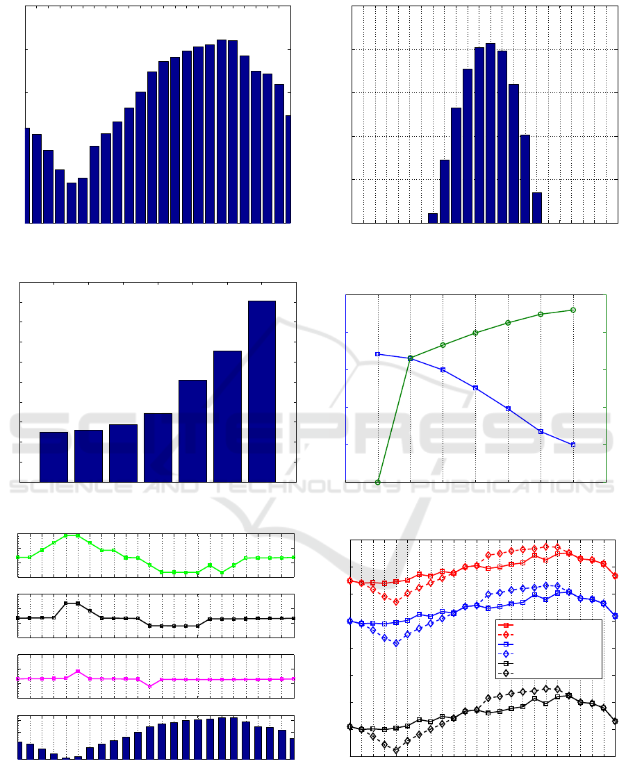
The simulation parameters are given in Table 1. We
use the historical data of the PJM day-ahead market
in our simulations, see Figure 4. We use the solar
radiation data from the National Solar Radiation
Data Base (National Renewable Energy Laboratory,
2015) as a proxy of the predicted renewable energy
generation. For simplicity, we assume that the
solar cell efficiency is 20%. The renewable energy
generation prediction is shown in Figure 5. We notice
that the solar power generation begins at 8:00 and
ends at 17:00 with a peak at 13:00.
6.1 DP Algorithm versus Greedy
Algorithm
We use the greedy algorithm as the benchmark, and
compare DP algorithm with the greedy algorithm.
Figure 6 shows the profit increase of DP algorithm
(using greedy algorithm as the benchmark). The
simulation reveals that DP algorithm achieves up
to 9% increase in profit in contrast to the greedy
algorithm. The reason why DP algorithm can achieve
a higher profit is that it exploits the information of
the entire hourly day-ahead prices and the renewable
energy prediction to make optimized decisions at each
horizon. The decisions made in each horizon are
optimized so that the aggregated profit over multiple
horizons is maximized. In contrast, the greedy
algorithm is a myopic algorithm because it only
maximizes the profit in the current horizon without
considering the day-ahead prices and the renewable
energy generation in the future. Comparing the
computational complexity of the two algorithms,
we note that greedy algorithm has a linear time
complexity O(N), while DP algorithm has a quadratic
time complexity O(N
2
), where N is the number of
planning horizons. Therefore, DP algorithm achieves
a higher profit (better performance) at the cost of
increased computing time.
6.2 Tradoff between Profit And
Customer Satisfaction
This section considers how the profit and customer
satisfaction change as the customer satisfaction
weighting parameter β increases from 0 to 30000 with
an interval of 5000. From Figure 7, we observe that
as β increases, the customer satisfaction increases
and the profit suffers a significant decrease. It
is clear that the charging service provider should
Dynamic Pricing and Energy Management Strategy for EV Charging Stations under Uncertainties
55

Table 1: Simulation Parameters.
Coefficient Description Unit Value
N Number of horizons - 24
E Energy storage capacity MWh 200
ω Customer satisfaction para. - 0.01
α Customer satisfaction para. - 5e-5
β Satisfaction Parameter - 0, ···, 30000
µ Power grid impact parameter - 0.1
η Storage cost $/MWh 0.5, 1.0, 1.5
o
ref
Reference purchase MWh 40
make a tradeoff between profit maximization and
customer satisfaction improvement by choosing a
proper weighting parameter β.
6.3 The Aggressive or Conservative
Electricity Purchase Strategy
The electricity storage system enables the charging
service provider to purchase extra electricity from the
wholesale market when the wholesale price is low,
and store the unsold electricity for future use when
the wholesale price is high. In this simulation, we
analyze how this “buy low and sell high” strategy
may change as the energy storage cost increases. In
Figure 8, the first three subplots are the electricity
purchase with different energy storage costs (η =
0.5,η = 1.0,η = 1.5 ), and the last subplot is the
day-ahead wholesale market prices. From Figure
8, we make three observations: (1) The average
electricity purchase is 37 MWh in each horizon; (2)
When η = 1.5, the electricity purchase almost does
not change. This suggests that the service provider
becomes conservative in electricity purchase as the
storage cost increase. In other words, the service
provider cannot improve the profit through “buy low
and sell high” strategy due to the high storage cost;
(3) When η = 0.5 and η = 1.0, the service provider
is likely to purchase more electricity during low-
price horizons (from 3:00 to 8:00), and purchase less
electricity during high-price horizons (from 11:00 to
19:00). Generally speaking, low electricity storage
cost spurs the service provider to adopt an aggressive
electricity purchase strategy.
6.4 Smoothing Price Fluctuation via
Electricity Storage System
In this section, we investigate the correlation between
the charging prices and the electricity storage cost. In
the simulation we have 20 charging stations in total,
and we randomly choose 3 charging stations to plot
Figure 9. The solid lines represent the charging prices
with low storage cost (η = 0.5), and the dash lines are
the charging prices with high storage cost (η = 1.5).
First, we notice that different charging stations
have different charging prices. Second, the charging
prices with high storage cost are more volatile than
those with low storage cost. When the wholesale
prices are low (from 1:00 to 8:00), the charging prices
with high storage cost are lower than those with low
storage cost. When the wholesale prices are high
(from 12:00 to 19:00), the charging prices with high
storage cost are higher than those with low storage
cost. The reason for the difference is that when the
storage cost is low, the service provider can have more
electricity reserved in the storage system which can be
used in the future when the wholesale electricity price
is high. Therefore, the charging prices stay relatively
stable over time. As the storage cost increases,
electricity storage becomes expensive. Without the
“buffer effect” of the electricity storage system, the
EV owners are exposed to the varying charging price
which is directly influenced by the wholesale market.
Hence, a low-cost energy storage system can not only
increase the total profit but also act as a buffer to
smooth out the fluctuation of the charging prices.
7 CONCLUSION
In this paper, a DP based pricing and energy
management framework for EV charging stations is
studied. The proposed framework aims to strike a
balance among three conflicting goals of improving
the total profit, enhancing the user satisfaction, and
reducing the EV charging impact on the power grid.
In this study here, we incorporate the electricity
storage system and the renewable energy generation
as an energy supplement. To solve the optimization
problem, we apply the DP algorithm to calculate the
charging prices and the electricity purchase for each
planning horizon. The simulation results show that
the DP algorithm can obtain higher profits compared
with the greedy algorithm. In addition, we observe
VEHITS 2016 - International Conference on Vehicle Technology and Intelligent Transport Systems
56

0 1 2 3 4 5 6 7 8 9 10 11 12 13 14 15 16 17 18 19 20 21 22 23
10
15
20
25
30
35
Time
Prices($\MWh)
Figure 4: PJM Electricity Wholesale Prices.
0
1
2
3
4
5
6
7
8
9
10
Profit Gain (Percentage)
β = 0
2.6%
2.9%
3.4%
5.1%
6.6%
9.1%
2.5%
β =5000
β = 10000
β = 15000
β = 20000
β = 25000 β = 30000
Figure 6: DP Profit Increase Percentage.
0 1 2 3 4 5 6 7 8 9 10 11 12 13 14 15 16 17 18 19 20 21 22 23
10
30
50
70
η=0.5
Purchase(MWh)
0 1 2 3 4 5 6 7 8 9 10 11 12 13 14 15 16 17 18 19 20 21 22 23
10
30
50
70
η=1.0
Purchase(MWh)
0 1 2 3 4 5 6 7 8 9 10 11 12 13 14 15 16 17 18 19 20 21 22 23
10
30
50
70
η=1.5
Purchase(MWh)
0 1 2 3 4 5 6 7 8 9 10 11 12 13 14 15 16 17 18 19 20 21 22 23
15
20
25
30
Time
Prices($/MWh)
Figure 8: Electricity Purchase with Different Storage Cost.
that the electricity purchase is heavily influenced by
the wholesale prices and the energy storage cost.
A low-cost energy storage system is beneficial for
0 1 2 3 4 5 6 7 8 9 10 11 12 13 14 15 16 17 18 19 20 21 22 23
0
5
10
15
20
25
Time
Renewable energy (MWh)
Figure 5: Hourly Renewable Energy Generation.
0
2
4
6
8
10
x 10
4
Profit
0
0.1
0.2
0.3
0.4
0.5
Customer satisfaction
β = 0
β =5000
β = 10000
β = 15000
β = 20000 β = 25000
β = 30000
Figure 7: Total Profit vs Customer Satisfaction.
0 1 2 3 4 5 6 7 8 9 10 11 12 13 14 15 16 17 18 19 20 21 22 23
62
64
66
68
70
72
74
76
78
Time
Prices($/MWh)
Charging station 7, η=0.5
Charging station 7, η=1.5
Charging station 18, η=0.5
Charging station 18, η=1.5
Charging station 21, η=0.5
Charging station 21, η=1.5
Figure 9: Charging Prices with Different Storage Cost.
improving the profit and stabilizing the charging
prices.
Dynamic Pricing and Energy Management Strategy for EV Charging Stations under Uncertainties
57

ACKNOWLEDGEMENTS
This work has been partially supported by the
National Science Foundation under grants CNS-
1239224, ECCS-1550016, and CPS-1544724.
REFERENCES
Ban, D., Michailidis, G., and Devetsikiotis, M. (2012).
Demand response control for phev charging stations
by dynamic price adjustments. 2012 IEEE PES
Innovative Smart Grid Technologies, pages 1–8.
Bertsekas, D. (2000). Dynamic Programming and Optimal
Control (2nd ed.). Athena Scientific, Belmont,
Massachusetts.
Cormen, T., Leiserson, C., Rivest, R., and Stein, C. (2001).
Introduction to Algorithm (2nd ed.). MIT Press &
McGraw-Hill.
Electric Drive Transportation Association (2015). Electric
drive sales dashboard. Available at: http://
electricdrive.org/index.php?ht=d/sp/i/20952/pid/
20952. [Online].
Fahrioglu, M., Fern, M., and Alvarado, F. (1999). De-
signing cost effective demand management contracts
using game theory. Proc. of IEEE Power Engineering
Society 1999 Winter Meeting, 1:427–432.
Faranda, R., Pievatolo, A., and Tironi, E. (2007). Load
shedding: A new proposal. IEEE Transactions on
Power Systems, 22(4):2086–2093.
Frame, J. (2001). Locational marginal pricing. 2001 IEEE
Power Engineering Society Winter Meeting 2001,
1:377–382.
Guo, Y., Liu, X., Yan, Y., Zhang, N., and Su, W. (2014).
Economic analysis of plug-in electric vehicle parking
deck with dynamic pricing. 2014 IEEE Power and
Energy Society General Meeting, pages 1–5.
Guo, Y., Xiong, J., Xu, S., and Su, W. (2016). Two-stage
economic operation of microgrid-like electric vehicle
parking deck. accepted by IEEE Transactions on
Smart Grid (to appear).
Han, Y., Chen, Y., Han, F., and Liu, K. J. R. (2012). An
optimal dynamic pricing and schedule approach in
v2g. Proceedings of The 2012 Asia Pacific Signal and
Information Processing Association Annual Summit
and Conference, pages 1–8.
Huisman, R., Huurman, C., and Mahieu, R. (2007).
Hourly electricity prices in day-ahead markets.
SciVerse ScienceDirect Journals, Energy Economics,
29(2):240–248.
IEC (2007). Efficient electrical energy transmission and
distribution. Available at: http://www.iec.ch/news
centre/onlinepubs/pdf/transmission.pdf. [Online].
Kinter-Meyer, M., Schneider, K., and Pratt, R. (2007).
Impacts assessment of plug-in hybrid electric vehicles
on electric utilities and regional u.s. power grids: Part
i:technical analysis. Online Journal of EUEC, 1.
Lopes, J., Soares, F., and Almeida, P. (2011). Integration
of electric vehicles in the electric power system.
Proceedings of the IEEE, 99(1):168 – 183.
Martirano, D. L., Devetsikiotis, M., and Pietra, B. (2014).
Interactive energy: an approach for the dynamic
pricing and dispatching of ev charging service. The
40th Annual Conference of the IEEE - Industrial
Electronics Society, IECON 2014, pages 3556–3562.
National Renewable Energy Laboratory (2015). Na-
tional solar radiation data base. Available at:
http://rredc.nrel.gov/solar/old data/nsrdb/. [Online].
Navigant Research (2014). Electric vehicle market
forecasts global forecasts for light duty hybrid,
plug-in hybrid, and battery electric vehicle sales
and vehicles in use: 2014-2023. Available at:
http://www.navigantresearch.com/research/electric-
vehicle-market-forecasts. [Online].
Nemhauser, G. (1996). Introduction to Dynamic
Programming. John Wiley and Sons, Inc.
Proakis, J. (2007). Digital Signal Processing (4th ed.).
Pearson Prentice Hall, Upper Saddle River, N.J.
Rahbari-Asr, N., Chow, M.-Y., Yang, Z., and Chen, J.
(2013). Network cooperative distributed pricing
control system for large-scale optimal charging of
phevs/pevs. The 39th Annual Conference of the IEEE
- Industrial Electronics Society, IECON 2013, pages
6148–6153.
Scott, M., Kintner-Meyer, M., Elliott, D., and Warwick, W.
(2007). Economic assessment and impacts assessment
of plug-in hybrid vehicles on electric utilities and
regional u.s. power grids. part ii. Online Journal of
EUEC, 1.
Simpson, A. (2006). Cost-benefit analysis of plug-
in hybrid electric vehicle technology. The 22nd
International Battery, Hybrid and Fuel Cell Electric
Vehicle Symposium and Exhibition (EVS-22).
Treinen, R. (2005). Locational marginal pricing (lmp):
Basics of nodal price calculation. Available
at: http://www.caiso.com/docs/2004/02/13/
200402131607358643.pdf. [Online].
Yan, Q., Manickam, I., Kezunovic, M., and Xie, L. (2014).
A multi-tiered real-time pricing algorithm for electric
vehicle charging stations. 2014 IEEE Transportation
Electrification Conference and Expo, pages 1–6.
Yang, P., Tang, G., and Nehorai, A. (2013). A game-
theoretic approach for optimal time-of-use electricity
pricing. IEEE Transactions on Power Systems,
28(2):884–892.
APPENDIX
Given the following optimization problem
J
k
(I
k
) =
max
P
k
,o
k
,···,P
N
,o
N
(
Π
N+1
(I
N+1
) +
N
∑
j=k
Π
j
(I
j
,P
j
,o
j
)
)
.
(23)
VEHITS 2016 - International Conference on Vehicle Technology and Intelligent Transport Systems
58

Note that I
j+1
= I
j
+ u
j
+ o
j
− φ
j
;( j > k), so I
j+1
is
a function of I
j
,o
j
,and P
j
. We can prove that I
j+1
is actually a function of (I
k
,o
k
,o
k+1
,o
j
,P
k
,··· ,P
j
) by
recursively applying the formula to substitute I
j
. Then
we can rewrite Equation (23) as follows,
J
k
(I
k
) = max
P
k
,o
k
,···,P
N
,o
N

Π
N+1
(I
N+1
)+
N
∑
j=k
Π
j
(I
k
,P
k
,··· ,P
j
,o
k
,··· ,o
j
)

= max
P
k
,o
k
(
Π
k
(I
k
,P
k
,o
k
)+
max
P
k+1
,o
k+1
,···,P
N
,o
N

Π
N+1
+
N
∑
j=k+1
Π
j

)
= max
P
k
,o
k

Π
k
(I
k
,P
k
,o
k
) + J
k+1
(I
k+1
)

,
(24)
where J
k+1
(I
k+1
) is given by
J
k+1
(I
k+1
) = max
P
k+1
,o
k+1
,···,P
N
,o
N
(
Π
N+1
+
N
∑
j=k+1
Π
j
)
.
(25)
Dynamic Pricing and Energy Management Strategy for EV Charging Stations under Uncertainties
59