Usability of Passive Models for Energy Minimization of
Transcutaneous Electrical Stimulation
Possibilities and Shortcomings of Analytical Solutions of Passive Models and
Possible Improvements
Aljoscha Reinert, Jan C. Loitz, Nils Remer, Dietmar Schroeder and Wolfgang H. Krautschneider
Institute of Nano- and Medical Electronics, Hamburg University of Technology, Eissendorfer Str. 38, Hamburg, Germany
Keywords:
Transcutaneous Electrical Stimulation, Passive Model, Active Model, Energy, Minimization.
Abstract:
Transcutaneous electrical stimulation is a more and more used rehabilitation technique for patients suffering
from spinal cord injury or stroke. The commonly used pulse shape is the biphasic rectangular pulse, which
leads to the question whether another, more efficient pulse shape exists that consumes less energy. In this
study a passive model for electrical stimulation was develepod and an analytical analysis was performed. The
resulting energy optimal pulse shape was then compared to the results of an active model. To improve the
accuracy of the passive model, a simple ionic current correction was introduced, which leads to comparable
results of an active model. Concluding it can be said that passive models are a good approach to give notions
of some effects, but have to be extended to fit reality.
1 INTRODUCTION
Transcutaneous electrical stimulation (TES) is known
to be used as a rehabilitation technique for patients
suffering from spinal cord injury or stroke since
the 1970s (Knutson et al., 2007). The most com-
monly used pulse shape for electrical stimulation
is the biphasic rectangular pulse with a short inter-
phase with the attributes stimulation amplitude (mA),
pulse duration (µs) and stimulation frequency (Hz)
(Hunter Peckham, 1999). The relation between am-
plitude and duration for energy optimized stimulation
with rectangular pulses is shown in the strength dura-
tion curve for biphasic rectangular pulses. As modern
electronics allow not only to change amplitude, dura-
tion and frequency, but also the shape of the stimu-
lation pulse, the question occurred whether it is pos-
sible to find an optimized pulse shape that consumes
the least energy.
This question was discussed several times in the
past (Jezernik and Morari, 2005; Wongsarnpigoon
and Grill, 2010; Krouchev et al., 2014). Most of these
papers do not differentiate between the energy that
has to be provided by the battery of the stimulator and
the energy that is applied to the patient. This paper fo-
cuses on the energy transmitted to the patient, as the
possible harm for the body should be minimized. It
should also be noted that the optimal pulse shape is
one single shape, with a distinct amplitude, as bound-
ary conditions like maximum amplitude or fixed pulse
duration contradict the definition of energy optimized.
The goal of this study is to develop a passive
model, i.e. based only on capacitors and resistors,
to find an analytical solution and to figure out how
this solution can be used for the prediction of action
potentials. In the second step this passive model is
compared to an active model, which uses differential
equations to model the ionic current in the axon. In
the third step we investigate how the passive model
can be improved to match the active model without
dramatic increment of complexity.
2 PASSIVE MODEL
2.1 Development of a Passive Model
For transcutaneous electrical stimulation a lot of dif-
ferent models with varying complexity are available
(Kuhn and Keller, 2005; Kuhn et al., 2009; Villarreal
et al., 2013). Those equivalent circuits are often built
as passive models, only consisting of capacitors and
resistors, as electrical parameters are known and sim-
ulating passive models is very fast and accurate. In
the following, the development of an equivalent cir-
Reinert, A., Loitz, J., Remer, N., Schroeder, D. and Krautschneider, W.
Usability of Passive Models for Energy Minimization of Transcutaneous Electrical Stimulation - Possibilities and Shortcomings of Analytical Solutions of Passive Models and Possible
Improvements.
DOI: 10.5220/0005822402690274
In Proceedings of the 9th International Joint Conference on Biomedical Engineering Systems and Technologies (BIOSTEC 2016) - Volume 1: BIODEVICES, pages 269-274
ISBN: 978-989-758-170-0
Copyright
c
 2016 by SCITEPRESS – Science and Technology Publications, Lda. All rights reserved
269

cuit for the prediction of triggering an action potential
is described.
The simplest equivalent circuit model of the axon
is shown in figure 1. It consists solemnly of one RC-
circuit, which is the merged form of two serial RC-
circuits (one for entering the axon, one for leaving the
axon) with the same electrical properties. The axon
membrane is represented by the capacitor as all leak-
age currents and surrounding tissue is merged into the
parallel resistor. In this model the current path from
the electrodes to the axon is neglected. It can easily
be seen that this is a simplification that dramatically
changes the reliability of the results. Therefore this
model has to be extended.
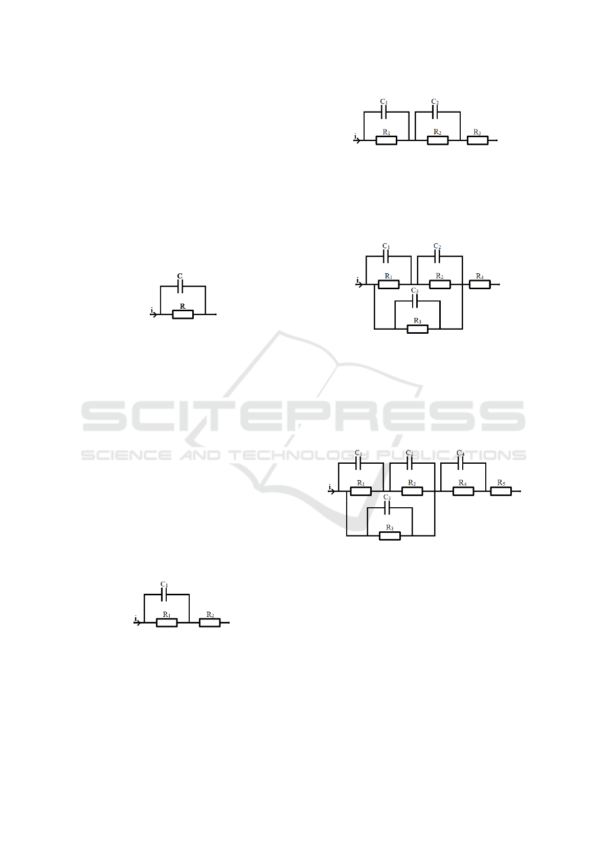
Figure 1: Most simple passive model of an axon, consisting
only of a membrane capacitor and resistor.
To include the losses in the current path between
electrodes and axon, another series resistor (R
2
) has
been added. The corresponding equivalent circuit is
shown in figure 2. The resistor R
2
merges the resis-
tive losses of the current path to and from the axon, as
the two serial resistors for both paths can be merged
into one resistor. The same is true for all following
models and their serial impedance. The added resis-
tor dramatically changes the behavior of the model,
but it is still not quite accurate. In this model there is
still the assumption that all of the stimulation current
is flowing through the axon and the surrounding tis-
sue, neglecting a possible current path, which is close
to the electrodes, far away from the axon. This is
also a simplification as all losses in the electrode skin
interface is neglected, which can be extremely high
because of the high electrode size when performing
transcutaneous electrical stimulation.
Figure 2: Passive model that considers losses in cables and
tissue.
To consider this interface and the capacitive be-
havior of the tissue another series RC circuit (R
2
C
2
)
has been added, as shown in figure 3.
The amount of current that flows into the tissue
and passes the tissue around the axon can be consid-
ered by adding an additional RC circuit in parallel to
Figure 3: Passive model that considers the electrode-skin-
interface and capacitive behavior of tissue.
the existing RC-circuits (R
3
C
3
). The amount of cur-
rent that does not enter the path required for stimula-
tion is determined by the impedance ratio of the two
parallel paths, shown in figure 4.
Figure 4: Passive model that considers the capacitive behav-
ior of tissue and the distribution between current that flows
through the axon and current that does not.
As the electrode skin interface and tissue behavior
can no longer be merged together into one RC-circuit,
the last step is to add another series RC circuit to the
existing schematic to model the electrode skin inter-
face and tissue path to the axon (R
4
C
4
), see figure 5.
Figure 5: Passive model that considers the electrode-skin-
interface,capacitive behavior of tissue and current distribu-
tion.
This model can now be extended with additional
RC-circuits that represent single layers of skin, fat or
muscle, forming an RC-network. For a given fre-
quency this network can always be simplified to the
last step of the model given in figure 5. All these mod-
els focus on predicting action potentials of a single
node of Ranvier in the axon, therefore ignoring contri-
bution of neighboring cells that can be modeled with
the activating function (Rattay, 1999). Also only the
membrane potential is calculated as this is necessary
to decide whether or not an action potential is trig-
gered. The prediction stops at the moment when an
action potential is triggered, as the differential equa-
BIODEVICES 2016 - 9th International Conference on Biomedical Electronics and Devices
270

tions needed to describe an action potential (Hodgkin
and Huxley, 1952; McIntyre et al., 2002) and their re-
sulting ionic currents are not included in passive mod-
els.
2.2 Analytical Solutions for Energy
Minimization
When finding the optimal pulse shape, it is neces-
sary to minimize the energy for a fixed change of the
membrane potential V
m
or to maximize the change
of the potential V
m
with a fixed amount of energy E.
The third option would be maximizing the efficiency,
therefore maximizing
V
m
E
. This includes minimizing
the energy and maximizing the membrane potential
at the same time. In this paper the focus lies on the
energy that is dissipated in the tissue, not the energy
that is provided by the battery of the stimulator. As for
most stimulation devices a constant voltage source is
used, which gives for the latter
E =
Z
V
source
· i dt = V
source
· Q (1)
as V
source
is constant. Optimizing this means optimiz-
ing for charge, as the energy is only determined by the
integral of the current.
Calculating the energy in the tissue is given by a
varying voltage and current. Choosing the first model,
shown in figure 1, gives us the following equations.
The solution is straight-forward. As the voltage drop
over the membrane is determined by
i
C
= C ·
dV
m
dt
(2)
and the energy loss over the resistor is proportional to
the time
E
R
=
Z
V
m
· i
R
dt (3)
an infinitely high and infinitely short current spike is
the optimal solution. This would lead to an instanta-
neous voltage spike over the membrane capacitance
and therefore immediately trigger an action potential
without any losses over the resistor R.
Adding the series resistor in the second model in-
validates this solution, as the power loss in the series
resistor can be calculated by
E
R2
=
Z
i
2
· R
2
dt (4)
thereby limiting the maximum amplitude of the cur-
rent, as energy scales with the square of the current.
The efficiency is defined as:
dV
m
dE
=
dV
m
d
R
(V
m
· i + i
2
· R
2
) dt
(5)
Differentiating this equation and setting it equal to
zero will give us the maximums and minimums and
therefore the point of optimal energy efficient stimu-
lation. Doing this will lead to a complex differential
equation, where solving with Laplace leads to a con-
volution of the current i with an exponential function
e
−
t
τ
, which is very complex to solve analytically, as
the current itself is unknown. The solution however
is reasonable, as a convolution with an exponential
function is nothing else than the charge stored in the
capacitor, depending on the shape of the pulse and the
time elapsed.
To avoid this problem a minimization approach
for constant currents and infinitesimal time interval
has been chosen. The system is at every instant de-
fined by the charges stored in the capacitors and their
corresponding voltages. Applying an external con-
stant current I
1
to the system for a duration of dt will
lead to a change of the system state. At the point t +dt
the system a new constant current I
2
can be applied
to the system. For each single point in time the effi-
ciency can be calculated by using the current state of
the system. Always choosing the current I with the
highest efficiency for every single point then leads to
the energy optimized pulse shape i.
Following this logic claims that only one optimal
pulse shape exists. This is true as long as no addi-
tional boundary conditions are applied. In literature
the maximum amplitude or maximum pulse duration
is often applied as an additional boundary condition,
which can lead to different, less efficient results. Set-
ting the pulse duration to a predefined value is crit-
ical only if this value is too small, changing the ap-
pearance of the shape. A longer pulse duration only
leads to a shift of the optimized shape (Sahin and Tie,
2007).
As stated above, the first step is to find the most ef-
ficient waveform, which is given by maximizing
dV
m
dE
.
The voltage drop along the R
1
C
1
circuit in figure 2
can be calculated as:
V
1
= (V
0
− R
1
I) · e
−t
R
1
C
1
+ R
1
I (6)
V
0
defines the voltage drop at the capacitor at t = 0.
The voltage drop over the resistor R
2
is defined as
V
2
= R
2
I (7)
The assumption that for each given voltage an optimal
current exists is only valid for an infinite short amount
of time dt, which leads to the optimization problem of
maximizing the efficiency
X =
dV
dt
dE
dt
=
dV
dt
P
(8)
The power can be calculated by the product of volt-
age and current. Minimization of this equation with
Usability of Passive Models for Energy Minimization of Transcutaneous Electrical Stimulation - Possibilities and Shortcomings of
Analytical Solutions of Passive Models and Possible Improvements
271

respect to I leads to
I(V
1
) =
V
1
R
1
+V
1
s
R
1
+ R
2
R
2
1
R
2
(9)
Combining this equation with the original equa-
tion for the voltage drop then gives us a solution with
the shape of i = k · e
t
τ
. The result of an exponential
function as an optimal pulse shape for passive mod-
els has also been derived by (Wongsarnpigoon et al.,
2010). Adding additional RC-circuits as shown in in
figure 5, does not change the linearity of the differen-
tial equations, always leading to a result in the shape
of
i = Σ k
n
· e
t
τ
n
, k
n
≥ 0 (10)
Therefore passive models will always lead to expo-
nentially shaped pulse shapes as an optimal result, no
matter how many and detailed RC circuits are added.
However, experiments like (Wongsarnpigoon
et al., 2010) already showed that the exponential in-
crease is not the optimum pulse shape in reality. We
can conclude that there is still something important
missing, making passive models as they are right now
insufficient for the prediction of action potentials.
3 ACTIVE MODEL
3.1 Active Model Simulation Results
To build models that are closer to reality, the ionic
currents and active behavior of axons have to be mod-
eled as well. Active models that use the differen-
tial equations proposed by (McIntyre et al., 2002) are
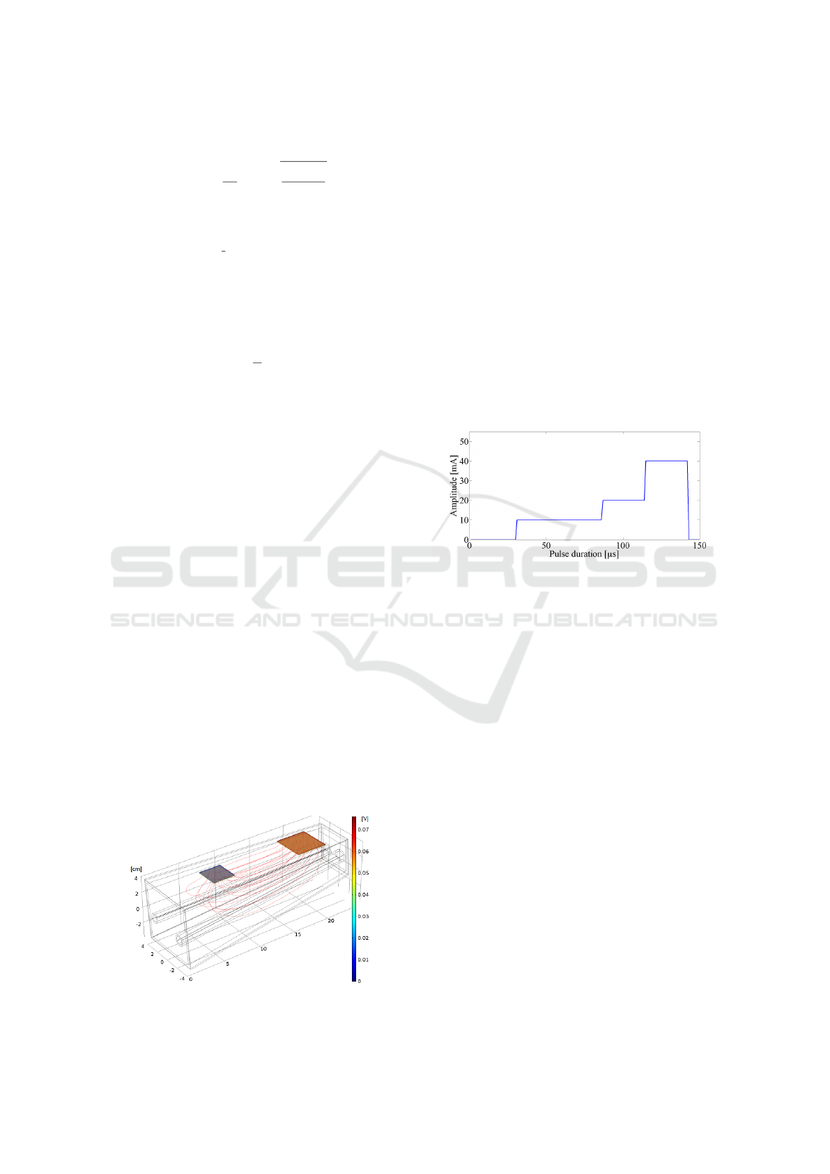
used to determine this behavior. As a basis for cal-
culation a 3D finite element (FE) model was used to
model the forearm and calculate the extracellular po-
tentials (Loitz et al., 2015) and is shown in figure 6.
To minimize calculation time, the system response to
Figure 6: Simplified finite element COMSOL model of a
human forearm.
a rectangular pulse of 1 mA and 1 µs was simulated in
COMSOL and post-processed in Matlab. This pulse
was then extended to 80 µs and the amplitude was var-
ied until the minimum amplitude to trigger an action
potential was found. This amplitude was set as the
maximum for the following steps. The duration of
80 µs was extended to 160 µs and split into multi-
ple segments as shown in figure 7. To keep calcula-
tion time low, a number of four segments was chosen.
For each of this rectangular segments the amplitude
was varied from minimum to maximum in steps of
10% of the maximum amplitude until an action po-
tential was triggered. All the valid results are then
compared and the solution with the least amount of
consumed energy was saved. This can be used as a
first approach to determine the optimal pulse shape.
Using only the electrical parameters from COMSOL
Figure 7: Finite Element Simulation results with Passive
Model and split pulse.
and applying the results to Matlab gives a roughly ex-
ponential shape as a result for an optimal pulse shape,
supporting the analytical solution found with the pas-
sive model as shown in figure 7. Now adding the
Hodgkin-Huxley equations to this model leads to an
interesting effect of decreasing current for the last of
the four rectangular pulses, see figure 8. This can be
explained with the ionic current that starts to flow be-
fore threshold is reached, therefore contributing to the
total current needed for stimulation. As the ionic cur-
rent can be calculated with the Hodgkin-Huxley equa-
tions and is approximately exponential at the begin-
ning it decreases the amount of external current that
is needed. This effect can be made more clear by in-
creasing the amount of segments from four to a higher
value, smoothing the shape of the stimulation pulse.
On the other hand this dramatically increases the sim-
ulation time, as all combinations of amplitudes have
to be computed and compared. (Meza-Cuevas et al.,
2012) experimentally showed that a pulse shape with
decreasing amplitude like sinusoidal is suited best to
trigger an action potential.
BIODEVICES 2016 - 9th International Conference on Biomedical Electronics and Devices
272

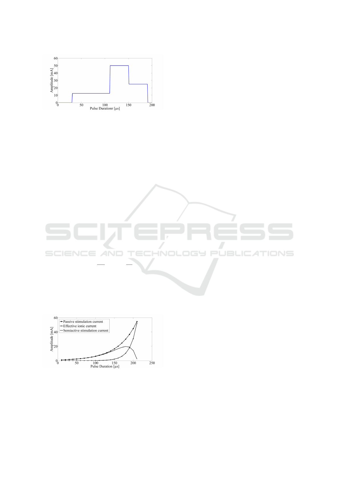
Figure 8: Finite Element Simulation results with Active
Model.
3.2 Semi-Active Model
To improve the passive models in a way that they can
be used to accurately predict action potentials an ex-
tension is needed. As this extension can no longer
be passive, the proposal is to use semi-active models.
These models are based on passive models, but have
a single, very limited active component, that can be
computed after the passive solution. Looking at the
Hodgkin-Huxley equations, it is possible to approx-
imate the behavior of the ionic current at the begin-
ning of the stimulation with an exponential increas-
ing function. After reaching the threshold potential
this approximation is no longer valid as the additional
ionic currents now dominate. The proposal is to in-
clude the ionic current as a fixed, exponentially in-
creasing current, that has to be subtracted from the
stimulation current, leading to a shape that can be ap-
proximately written as:
i = k
stim
· e
t
τ
stim
− k
ion
· e
t
τ
ion
(11)
The given equation consists of the stimulation current
and the ionic current that can be scaled to match the
optimization problem and gives fast results that are
comparable to those of an active model as shown in
figure 9. The passive stimulation current is given by
Figure 9: Exponential increase pulse with ionic current and
their difference.
the result of the passive model. The effective ionic
current is the representative current that has to be sub-
tracted from the external stimulation current to cause
the same effects as the internal ionic current.
As only a small amount of stimulation current
flows through the axon the magnitudes of the real
ionic current and the effective ionic current differ a
lot. To determine the parameters k
i
on and τ
i
on two
fixed points are needed. The first fixed point is at
the end of the stimulation, as the active ionic current
is now high enough to carry the action potential all
by itself, being equal to the equivalent passive model
external stimulation current. This results in a semi-
active stimulation current of zero at the end of the
pulse. The second point determines the maximum
of the semiactive pulse shape and is in the range of
50% to 80% of the pulse duration, depending on the
model. Determination of the exact position has to be
investigated further, a value of 66% showed very good
results and is recommended.
4 CONCLUSIONS
In this study a passive model with stepwise increas-
ing complexity has been developed that enables pre-
diction of action potentials with given pulse shapes
and allows to analytically calculate the optimal pulse
shape for energy minimization in the tissue. The re-
sults of these passive models are always exponen-
tially increasing shaped pulses. Comparing these
results with experiments leads to the problem that
even though passive models already lack the ability
to model the behavior during an action potential, they
also fail to accurately model the behavior shortly be-
fore an action potential is triggered. To improve the
passive model, a scalable ionic current has been intro-
duced that represents the behavior of the ion channels.
With these both combined results that are comparable
to these of an active model can be achieved. Passive
models are therefore a good way to quickly get a no-
tion of some effects, as this approach shows that the
results of an active and passive model may differ, but
never in a completely different way.
ACKNOWLEDGEMENTS
This work was supported by a grant from the Fed-
eral Ministry of Education and Research (BMBF, ES-
iMED [16M3201]).
REFERENCES
Hodgkin, A. L. and Huxley, A. F. (1952). A quantitative
description of membrane current and its application to
Usability of Passive Models for Energy Minimization of Transcutaneous Electrical Stimulation - Possibilities and Shortcomings of
Analytical Solutions of Passive Models and Possible Improvements
273

conduction and excitation in nerve. The Journal of
physiology, 117(4):500–544.
Hunter Peckham, P. (1999). Principles of electrical stim-
ulation. Topics in spinal cord injury rehabilitation,
5(1):1–5.
Jezernik, S. and Morari, M. (2005). Energy-optimal elec-
trical excitation of nerve fibers. Biomedical Engineer-
ing, IEEE Transactions on, 52(4):740–743.
Knutson, J. S., Harley, M. Y., Hisel, T. Z., and Chae, J.
(2007). Improving hand function in stroke survivors:
a pilot study of contralaterally controlled functional
electric stimulation in chronic hemiplegia. Archives of
physical medicine and rehabilitation, 88(4):513–520.
Krouchev, N. I., Danner, S. M., Vinet, A., Rattay, F.,
and Sawan, M. (2014). Energy-optimal electrical-
stimulation pulses shaped by the least-action princi-
ple. PloS one, 9(3).
Kuhn, A. and Keller, T. (2005). A 3d transient model for
transcutaneous functional electrical stimulation. In
International functional electrical stimulation society
conference, volume 10, pages 385–387.
Kuhn, A., Keller, T., Lawrence, M., and Morari, M. (2009).
A model for transcutaneous current stimulation: sim-
ulations and experiments. Medical & biological engi-
neering & computing, 47(3):279–289.
Loitz, J. C., Reinert, A., Schroeder, D., and Krautschnei-
der, W. H. (2015). Impact of electrode geometry on
force generation during functional electrical stimula-
tion. Current Directions in Biomedical Engineering,
1(1):458–461.
McIntyre, C. C., Richardson, A. G., and Grill, W. M.
(2002). Modeling the excitability of mammalian nerve
fibers: influence of afterpotentials on the recovery cy-
cle. Journal of neurophysiology, 87(2):995–1006.
Meza-Cuevas, M., Schroeder, D., Krautschneider, W. H.,
et al. (2012). Neuromuscular electrical stimulation
using different waveforms: Properties comparison by
applying single pulses. In Biomedical Engineering
and Informatics (BMEI), 2012 5th International Con-
ference on, pages 840–845. IEEE.
Rattay, F. (1999). The basic mechanism for the electri-
cal stimulation of the nervous system. Neuroscience,
89(2):335–346.
Sahin, M. and Tie, Y. (2007). Non-rectangular waveforms
for neural stimulation with practical electrodes. Jour-
nal of neural engineering, 4(3):227.
Villarreal, D. L., Schroeder, D., , and Krautschneider, W. H.
(2013). Equivalent Circuit Model to Simulate Neu-
rostimulation by using Different Waveforms. In ICT
Open 2013.
Wongsarnpigoon, A. and Grill, W. M. (2010). Energy-
efficient waveform shapes for neural stimulation re-
vealed with a genetic algorithm. Journal of neural
engineering, 7(4):046009.
Wongsarnpigoon, A., Woock, J. P., and Grill, W. M. (2010).
Efficiency analysis of waveform shape for electri-
cal excitation of nerve fibers. Neural Systems and
Rehabilitation Engineering, IEEE Transactions on,
18(3):319–328.
BIODEVICES 2016 - 9th International Conference on Biomedical Electronics and Devices
274