Resources Planning in Database Infrastructures

Eden Dosciatti

, Marcelo Teixeira

, Richardson Ribeiro

, Marco Barbosa

, F´abio Favarim

Fabr´ıcio Enembreck

and Dieky Adzkiya

Federal University of Technology-Paran´a, Pato Branco, Brazil

Pontiﬁcial Catholical University-Paran´a, Curitiba, Brazil

Delft University of Technology, Delft, The Netherlands

Keywords:

Modeling, Simulation, Resources Planning, Performance, Availability.

Abstract:

Anticipating resources consumption is essential to project robust database infrastructures able to support trans-

actions to be processed with certain quality levels. In Database-as-a-Service (DBaaS), for example, it could

help to construct Service Level Agreements (SLA) to intermediate service customers and providers. A proper

database resources assessment can avoid mistakes when choosing technology, hardware, network, client pro-

ﬁles, etc. However, to be properly evaluated, a database transaction usually requires the physical system to

be measured, which can be expensive an time consuming. As most information about resource consumption

are useful at design time, before developing the whole system, is essential to have mechanisms that partially

open the black box hiding the in-operation system. This motivates the adoption of predictive evaluation mod-

els. In this paper, we propose a simulation model that can be used to estimate performance and availability

of database transactions at design time, when the system is still being conceived. By not requiring real time

inputs to be simulated, the model can provide useful information for resources planning. The accuracy of the

model is checked in the context of a SLA composition process, in which database operations are simulated

and model estimations are compared to measurements collected from a real database system.

1 INTRODUCTION

Transaction processing is a crucial part of the de-

velopment of modern web systems, such as those

based on Service-Oriented Architecture (SOA), a new

paradigm to compose distributed business models. In

SOA, an entire transaction is usually composed by

distinct phases, such as networking, service process-

ing, database processing, third-part processing, etc.

For resources planning, it is usual that each particular

phase is individually approached. In this paper, we

concentrate on evaluating database transaction pro-

cessing, especially for SOA systems (although not

only), complementing previous results focused on the

other phases of SOA (Rud et al., 2007; Bruneo et al.,

2010; Teixeira et al., 2015).

In SOA, transactions are directly related to Qual-

ity of Service (QoS), and Service Level Agreements

(SLAs) are mechanisms used to legally express com-

mitments among service customers and providers

(Sturm et al., 2000). Performance and availability of

database operations are examples of clauses that can

be agreed in SLA, specially when the database itself

is provided as a service (DBaaS).

The effects of not being able to fulﬁll a database

SLA are many. This kind of transaction commonly

appears in the context of a service composition, as a

particular stage of an SOA application. Therefore, if it

fails to fulﬁll the metrics accorded in an SLA, this will

probably affect the overall web service behavior and,

as a consequence, the overall service orchestration, in

a ripple effect, breaching one or more SLAs. Thus,

for an entire SOA process, it is important to prevent

a database transaction to fail or, at least, to be able to

anticipate when it is susceptible to happen.

This task may not be so easy, as the ratio of load

variation in web applications can reach the order of

300% (Chase et al., 2001), making it difﬁcult to an-

ticipate QoS. What is observed is that applications

are entirely developed to be then stressed and mea-

sured, which can be quite expensiveandtime consum-

ing. Recent works have suggested that SOA QoS can

be estimated by modeling (Rud et al., 2007; Bruneo

et al., 2010; Teixeira et al., 2015), but they have ba-

sically focused on networking and processing stages,

assuming that database time consumption is implicit,

which may be a strong assumption, as illustrated in

(Teixeira and Chaves, 2011).

Dosciatti, E., Teixeira, M., Ribeiro, R., Barbosa, M., Favarim, F., Enembreck, F. and Adzkiya, D.

Resources Planning in Database Infrastructures.

In Proceedings of the 18th International Conference on Enterprise Information Systems (ICEIS 2016) - Volume 1, pages 53-62

ISBN: 978-989-758-187-8

In this paper, we propose a stochastic model-

ing approach to estimate performance and availability

of database transactions susceptible to intense work-

loads. By adopting Generalized Stochastic Petri Nets

(GSPNs) as modeling formalism, we construct a for-

mal structure that can be simulated and estimations

can be used to anticipate resource consumption of

database operations running under different load pro-

ﬁles. Based on these estimations, it is furthermore

shown how to construct, at modeling time, realistic

contracts for database transactions, which can be nat-

urally combined as part of the estimations provided

in works such as in (Rud et al., 2007; Bruneo et al.,

2010; Teixeira et al., 2015).

The main advantage of our approach is not requir-

ing real-time measurements nor the complete system

implementation to be simulated. These information

may not be available at design-time, when resources

allocation is conducted. Instead, the model supports

high level parameters collected from the Data Base

Management System (DBMS) and statistics collected

from samples of database query execution. For this

reason, database technology, infrastructure or particu-

lar type of operation to be simulated, are implicit into

the simulation scheme.

An example of a contract composition process is

presented to illustrate the proposed approach. Using

parts of a real database system and samples of rela-

tional database operations, we collect the input pa-

rameters to the model, which is then simulated and

estimations are collected. Afterwards, we validate

the estimations. This could be done by comparing

them to benchmark data. In this paper, however, we

are more interested on the uncertainty observed in the

real-time behavior of transactions, e.g., how transac-

tions behave when parameters change, or what is the

performance degradation when workload increases,

or what is the rate of requests queueing for a load pro-

ﬁle, etc. These informations are not directly available

from benchmarks, since they focus mostly on best and

worst cases, for example. To be possible to check

the accuracy of the proposed model so, we compare

its estimations to measurements collected from a real

database system. Results indicate that it is possible

to trace the real behavior keeping a stochastically-

reasonable average of 80% accuracy.

The paper is organized as follows: Section 2 dis-

cusses the related work; Section 3 introduces the basic

concepts of SOA, SLA and GSPN; Section 4 presents

the proposed GSPN model. Section 5 presents an ex-

ample and some ﬁnal comments are discussed in Sec-

tion 6.

2 RELATED LITERATURE

Performance of databases has been a concern since

the ﬁrstly proposed technologies and relational mod-

els (Elhardt and Bayer, 1984; Adams, 1985). From

the web advent, however, advanced features have

been combined to the existent DBMSs, attempting to

support emergent requirements such as parallelism,

distribution (Dewitt and Gray, 1992), object (Kim

et al., 2002) and service-orientation (Tok and Bres-

san, 2006), etc. Although the interest on new tech-

nologies has recently grown, it has become more and

more difﬁcult to estimate their behavior.

In particular, when a database is part of a service,

or when it is provided as a service itself, it is usu-

ally exposed to a highly variable and data-intensive

environment, which makes it critical to estimate its

QoS levels. In (Ranganathan et al., 1998), it has been

discussed the impact of radically different workload

levels on the database performance and how it be-

comes a concern when the database is immersed in

QoS-aware frameworks that require QoS guarantees

(Lin and Kavi, 2013). In general, the literature tackle

this concern using run-time policies to ﬁlter and bal-

ance the database load (Lumb et al., 2003; Schroeder

et al., 2006; Krompass et al., 2008). When connect-

ing business partnerships, however, the negotiation of

QoS criteria starts much earlier, at the service design

phase, as it is necessary to plan and compose SLA

clauses to be agreed.

An option to cover this gap is by adopting analytic

models. For example, in (Tomov et al., 2004) it has

been proposed a queuing network model to estimate

the response time of database transactions. Further-

more, in (Osman and Knottenbelt, 2012) it has been

compared the performance of different database de-

signs via modeling. Queue time is predicted by us-

ing heuristic rules in (Zhou et al., 1997). Besides

not being natively constructed for web environments,

this approaches are also predominantly deterministic,

which often does not match the characteristics of the

real web environments (Teixeira et al., 2011) and can

compromise the accuracy when estimating transac-

tions with variable workloads. In addition, they are

not usually ﬂexible enough to be quickly converted in

practical tools, or to be modiﬁed to analyze different

system orchestrations, etc.

Thus, the need for supporting database QoS es-

timation remains. This is a quite challenging task,

as web environments practically lack execution pat-

terns and can present highly variable workloads, mak-

ing it critical for a transaction to be estimated (Nicola

and Jarke, 2000). In the same way, it is conceivably

difﬁcult to ensure that database queries will execute

ICEIS 2016 - 18th International Conference on Enterprise Information Systems

quickly enoughto keep the process ﬂow, avoiding it to

be delayed more than expected (Reiss and Kanungo,

2005). The modeling approach to be presented in this

paper is an option to face these challenges and imple-

ment database resources planning.

3 RELATED CONCEPTS

SOA comprises a set of principles for software devel-

opment, fundamentally based on the concept of ser-

vice (Josuttis, 2008). A service is a self-contained

component of software that receives a request, pro-

cesses it, and returns an answer. Eventually, a par-

ticular step of a service execution involves to access

a database structure an process a data transaction. It

may happen that a database transaction is itself of-

fered as a service (DBaaS). In this case, the transac-

tion processing is even more critical, as it is suscepti-

ble to a data-intensive environment, and its behavior

becomes difﬁcult to be estimated.

In SOA, legal commitments on services, including

database transactions, are expressed by a mechanism

known as Service Level Agreements (SLA) (Sturm

et al., 2000). An SLA expresses obligations and rights

regarding levels of QoS to be delivered and/or re-

ceived. SLA clauses usually involve metrics such as

response time, availability, cost, etc., and also estab-

lish penalties to be applied when a delivered service

is below the promised standard (Raibulet and Mas-

sarelli, 2008).

In practice, ensuring that a SOA system will be-

have as expected is very difﬁcult, and so it is difﬁcult

to compose, at design time, realistic SLAs. An alter-

native to probabilistically estimate the behavior of a

service is given by modeling approaches. A model

enables to observe the service behavior under “pres-

sure”, without exactly constructing the whole system.

The model described in this paper serves to this

purpose and it is modeled by Petri nets. Petri net

(PN) (Reisig and Rozenberg, 1998) is a formalism

that combines a mathematical foundation to an in-

tuitive modeling interface that allows to model sys-

tems characterized by concurrency, synchronization,

resources sharing, etc. These features appear quite of-

ten in SOA systems, which make PNs a natural mod-

eling choice.

Structurally, a Petri net is composed by places

(modeling states), transitions (modeling state

changes), and directed arcs (connecting places and

transitions). To express the conditions that hold in a

given state, places are marked with tokens.

Extensions of Petri nets have been developed to

include the notion of time (Murata, 1989), which al-

lows to represent time-dependent processes, such as

communication channels, code processing, hardware

designs, system workﬂows, etc. Generalized Stochas-

tic Petri Nets (GSPNs) (Kartson et al., 1995), for ex-

ample, is an extension that combines timed and non-

timed PNs. In GSPN, time is represented by random

variable, exponentially distributed, which are associ-

ated to timed transitions. When, for a given transi-

tion, the time is irrelevant, then one can simply use

non-timed (or immediate) transitions.

Formally, a GSPN is a 7-tuple GSPN = hP, T ,Π,

I, O,M,Wi, where:

• P = {p

, p

,.. ., p

} is a ﬁnite set of places;

• T = {t

,.. .,t

} is a ﬁnite set of transitions;

• Π : T → N is the priority function, where:

Π(t) =



≥ 1, if t ∈ T is immediate;

0, if t ∈ T is timed.

• I : (T × P) → N is the input function that deﬁnes

the multiplicities of directed arcs from places to

transitions;

• O : (T ×P) → N is the output function that deﬁnes

the multiplicities of directed arcs from transitions

to places;

• M : P→ N is the initial marking function. M indi-

cates the number of tokens

in each place, i.e., it

deﬁnes the state of a GSPN model;

• W : T → R

is the weight function that represents

either the immediate transitions weights (w

) or

the timed transitions rates (λ

), where:

W(t) =



≥ 0, if t ∈ T is immediate;

> 0, if t ∈ T is timed.

The relationship between places and transitions is

established by the sets

•

t and t

•

, deﬁned as follows.

Deﬁnition 1. Given a transition t ∈ T, deﬁne:

•

t = {p ∈ P | I(t, p) > 0} as the pre-conditions

of t;

• t

•

= {p ∈ P | O(t, p) > 0} as the post-conditions

of t.

A state of a GSPN changes when an enabled tran-

sition ﬁres. Only enabled transitions can ﬁre. Imme-

diate transitions ﬁre as soon as they get enabled. The

enabling rule for ﬁring and the ﬁring semantics are

deﬁned in the sequel.

Deﬁnition 2 (Enabling Rule). A transition t ∈ T is

said to be enabled in a marking M if and only if:

• ∀p ∈

•

t,M(p) ≥ I(t, p).

Black dots are usually used to graphically represent a token

in a place.

Resources Planning in Database Infrastructures

When an enabled transition ﬁres, it removes to-

kens from input to output places (its pre and post con-

ditions).

Deﬁnition 3 (Firing Rule). The ﬁring of transition t ∈

T enabled in the marking M leads to a new marking

′

such that ∀p ∈ (

•

t ∪ t

•

), M

′

(p) = M(p)−I(t, p)+

O(t, p).

A GSPN is said to be bounded if there exists a

limit k > 0 for the number of tokens in every place.

Then, one ensures that the state-space resulting from

a bounded GSPN is ﬁnite.

When the number of tokens in each input place

p of t is N times the minimum needed to enable t

(∀p ∈

•

t, M(p) ≥ N ×I(t, p), where N ∈ N and N > 1

), it enables the transition to ﬁre more than once. In

this situation, the transitiont is said to be enabled with

degree N > 0. Transition ﬁring may use one of the

following dynamic semantics:

• single-server: N sequential ﬁres;

• inﬁnite-server: N parallel ﬁres;

• k-server: the transition is enabled up to k times

in parallel; tokens that enable the transition to a

degree higher than k are handled after the ﬁrst k

ﬁrings.

It can be shown (Kartson et al., 1995; Marsan

et al., 1984) that GSPNs are isomorphic to

Continuous-Time Markov Chains (CTMC). However,

it is more expressive, as it allows to compute metrics

by both simulation and analysis of the state space. In

the last case, GSPN are indeed converted into CTMC

for analysis. Furthermore, GSPNs allow to combine

exponential arranges to model different time distribu-

tions (Desrochers, 1994), which is useful to capture

speciﬁc dynamics of systems.

4 PROPOSED MODEL

The modeling proposed in this paper starts when

a given web service requests a database operation.

When received in the DBMS, this request is buffered,

processed and buffered again, when an answer is

ready to be replied back to requestor. When this

happens, our modeling ﬁnishes. For this scenario,

we model the subphases of a database transaction in

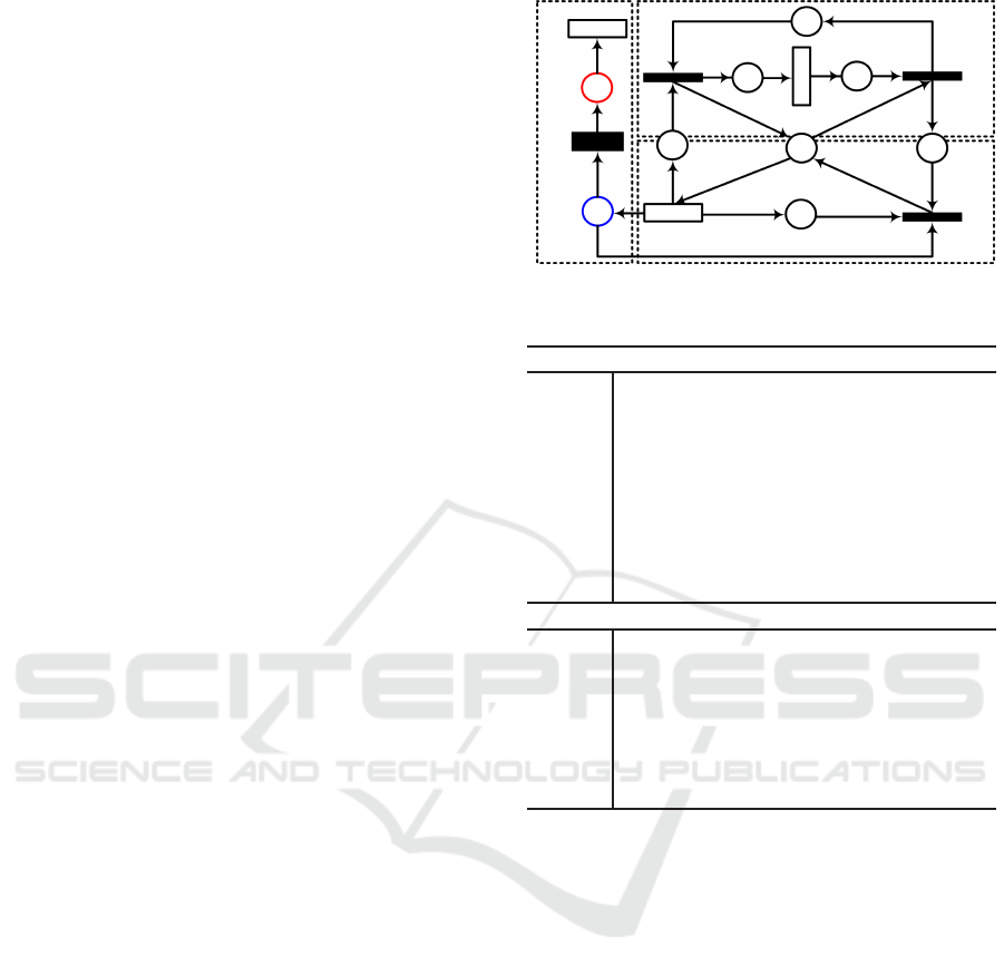
GSPN: Buffering and Processing, as shown in Fig. 1.

Table 1 summarizes the model’s notation.

Buffering Structure: The model ﬁrstly runs when

the timed transition T

ﬁres tokens toward the place

. Fired tokens model database requests and B

mod-

els the DBMS buffer. The ﬁring rate is deﬁned by

1/d

, where d

is the delay assigned to T

. The limit

(i)

(ii)

Exp

end

Processing

Buf fering

Timeout

Avail

Fail

end

SLA

Fail

IF(#P

= 0) : 0 ELSE 1

Figure 1: GSPN model.

Table 1: Notation of the GSPN model.

Places

Exp expectation of tokens to be processed;

resources available for buffering;

input buffer;

output buffer;

resources available for processing;

requests stored before processing;

requests stored after processing;

requests successfully attended;

requests that have failed.

Transitions

requests arrivals (delay d

);

requests processing (delay d);

SLA

requests failing (delay X

SLA

);

processing Input;

processing Output;

end

process exit point;

Fail

timeout exit point.

of tokens to be received in B

is controlled by the

number of tokens available in the place R

, which

are also shared with the output buffer B

. In order

to count the expectation of tokens into the model, and

consequently to be able to estimate their performance,

we create a place named Exp, that receives a copy of

each token arriving in the system, and loses a token

whenever the transition t

end

ﬁres.

Processing Structure: From B

, tokens are moved

to the place P

, which models the processing phase.

The place R

controls the number of requests that can

be concurrently processed. Tokens remain in P

long as it takes for them to be processed, which is

modeled by the delay d of the transition T

. After

processed, T

ﬁres moving tokens to P

from where

the immediate transition t

transfers them to the out-

put buffer B

. Remark that tokens leave the process-

ing phase if and only if there exist enough resources

in R

. On the contrary they remain in P

, waiting

for buffering resources. From B

, tokens immedi-

ately leave the model (by t

end

), which represents the

requestor being answered.

ICEIS 2016 - 18th International Conference on Enterprise Information Systems

Timeout Structure: When the transition T

ﬁrstly

ﬁres, besides to send a token to B

(performance

model), it also copies it in the place P

. The idea is to

be able to estimate how many requests delay longer

than a predeﬁned response time. For that purpose, we

assign to X

SLA

the time we intend to wait until count-

ing a failure. If the performance model reaches t

end

ﬁrst, P

loses the token and the transaction is success-

fully completed. If X

SLA

ﬁres ﬁrst, the transaction is

also completed (because the arc Avail gets 0), but a

failure is registered, i.e., a token reaches P

Repository of Resources: Two repository com-

prise our model: R

(buffering resources) and R

(processing resources). From/to R

and R

, we con-

nect arcs representing the number of tokens simulta-

neously moved when a source transition ﬁres. We de-

note by IR

and IR

the resources consumption and

by OR

and OR

the resources refunding from/to R

and R

, respectively. We assume that the number of

tokens moved from/to the repositories is conservative.

Blocking: By sharing R

with two consumers,

and B

, we actually design a possibly blocking

model. In fact if B

consumes all resources in R

then tokens cannot leave the processing phase. At the

same time, T

cannot ﬁre any more tokens to B

and,

so, the model is deadlocked. We avoid this by assign-

ing two logical conditions ((i) and (ii)) to the arcs that

lead to the place B

, where:

(i) : IF (#R

< IR

) : 0 ELSE IR

;

(ii) : IF (#R

< IR

) : 0 ELSE 1.

The formulas (i) and (ii) are syntactically compli-

ant to the TimeNET tool, adopted in this paper. Essen-

tially, the condition (i) avoids the deadlock by ﬁring

even without enough resources in R

. When this

is the case, the condition (ii) assigns 0 to the arc that

leads to B

and the token leaves the system. In prac-

tice, this models a situation when the DBMS rejects

new transactions while the system is completely full,

but as soon as any request is processed, transactions

get to be received again.

4.1 Model Parameters

To be simulated, the GSPN model requires to be set

up with parameters that connect it to the behavior of

the system that has been modeled. We show in the

following how such parameters can be derived.

4.1.1 Buffering Parameters

We ﬁrst deﬁne a marking

for R

, i.e., the number

of resources available for buffering. This is deﬁned

“#” denotes the marking of a place p, for #p ∈ N.

according to the real buffer size, measured in the

DBMS. Remark that each DBMS deﬁnes a particu-

lar amount of memory to be used for database opera-

tions and this can be tuned. The parameters we have

to collect from the DBMS are:

• Memory Pages (M

): number of blocks of mem-

ory allocated for database operations;

• Memory Page Size (M

): amount of bytes as-

signed to each M

Remark that the greater the number of memory

pages, the faster is the transfer from disk to memory,

but the greater is rate of I/O communication, which is

usually time expensive. On the other hand, the larger

the memory page, the slower the transfer to memory.

As from

= M

· M

we have the amount of memory available to store

messages from/to the database system, then the mark-

ing of R

is such that

= Av

Once R

is marked, we model its resources con-

sumption by assigning weights to the arcs IR

and

. To deﬁne those values, we have to collect the

mean size (bytes) of:

• Ω

: messages received in the database system;

• Ω

Out

: messages produced by the system as an-

swer.

Thus, IR

= Ω

and OR

= Ω

Out

. Ω

and Ω

Out

can be derived from samples of database transactions.

After assigning #R

, IR

and OR

to the GSPN,

it becomes already possible to estimate the database

Buffering Response Time (B

), taking into account

the concept of Mean Response Time (M

). In Petri

net, M

results from the expectation (ξ) of marking

in a given place X (ξ(X)), with respect to: (i) the rate

(λ) of requests; or (ii) the delay (d) between requests,

i.e.,

(i) M

ξ(X)

or, equivalently,(ii) M

= ξ(X) · d.

Tools like TimeNET syntactically implement these

formulas respectively by

(i) M

= ξ(X)/λ and (ii) M

= E{#X} · d.

So, B

can be estimated as follows:

ξ(B

) + ξ(B

)

Note that λ simply results from 1/d

, where d

the delay of the timed transition T

. In practice, B

represents the average of time spent by transactions

before and after processing.

Resources Planning in Database Infrastructures

4.1.2 Processing Parameters

This phase starts when t

ﬁres tokens towards the

place P

, ﬁnishing when the transition t

releases

them. There are basically four processing parameters

to be derived: the delay d for the transition T

, the

marking for R

and the weights for the arcs IR

and

, which connect the model from/to the repository

of processing resources.

Marking R

requires to measure the system in or-

der to collect the major number of operations simul-

taneously supported by the DBMS, without queueing

requests. This can be done by gradually increasing the

workload of requests until the point where the system

starts to queue. This speciﬁc point can be detected

by a sudden increase in the response time, when the

processing resources are at all consumed.

Thus, #R

receives the value of the workload

applied before observing evidences of queue, and 1 is

assigned to the weight of the arcs IR

and OR

Processing Response Time (P

ξ(P

) + ξ(P

)

where, ξ(P

) and ξ(P

) are respectively the expecta-

tion of marking in P

and P

4.1.3 Database Mean Response Time

From B

and P

, one can estimate the overall

database M

by:

ξ(Exp)

or, equivalently, Σ

= B

+ P

5 MODEL ASSESSMENT

Consider the process shown in Fig. 2.

Interface

Orchestrator

Service

SLA

Buffer

DBMS

DB infrastructure

Figure 2: Evaluated Process.

The process starts when remote users invoke an

orchestration service, via a web browser. Requests

are organized according to the process workﬂow, and

prepared to access remote services, which may access

other services or interact with databases (dashed cir-

cle). Between a service and its consumer, a SLA reg-

ulates the QoS that is to be offered. Usually, this SLA

is empirically constructed and, as a consequence, it is

not rare to observe services delaying longer than the

minimum necessary to match their contracts, which

can entail legal penalties for providers, bad reputa-

tion for services, money loses for customers, and so

on. Our goal here is to anticipate the behavior of the

database service when it is variably accessed.

5.1 Database Construction

For the experiments that follow, we consider a partial

structure of a relational database system, composed

by the following structures:

•

PRODUCT

(ProdID, ProdDesc, ProdColor)

•

CLIENT

(CliID, CliName, CliAddress)

•

INVOICE

(InvID, InvDate, InvValue, ShipmentDate, DeadlineDate,

FKClient

)

– FKClient references CLIENT

•

MOVINVOICE

(Quant, Discount, UnitValue, Label, Status, FKInvoice

FKProduct

)

– FKInvoice references INVOICE,

– FKProduct references PRODUCT

In order to access the database, we implement the

following operations in Relational Algebra

C ← Π

∗

(Client)

I ← Π

∗

(Invoice)

M ← Π

∗

(MovInvoice)

P ← Π

∗

(Product)

Deﬁne query 1:

∗

( σ (I.ShipmentDate <=

′

10/08/2015

′

∧ I.DeadlineDate <=

′

11/05/2015

′

))

(C ⋊⋉ I ⋊⋉ M ⋊⋉ P)

Deﬁne query 2:

∆ ← Π

∗

(σ (M.UnitValue >= 5.000,00

∧ M.FKProduct = 23)) (M)

M ← Π Quant,Discount,UnitValue,Status,

Label ←

′

Profitable

′

(∆)

Deﬁne query 3:

Λ ← Π I.InvID,I.InvValue,P.ProdID,

′

Delayed

′

Sold

′

(σ (I.DeadlineDate <=

′

CurrentDate

′

∧ I.ShipmentDate >=

′

10/10/2015

′

∧ I.InvValue >= 100.000,00))

(I ⋊⋉ M ⋊⋉ P)

M ← M ∪ {Quant,Discount,Λ}.

Notation

∗

refers to all attributes from a relation.

ICEIS 2016 - 18th International Conference on Enterprise Information Systems

Query 1 returns the clients and their respective in-

voices, admitting that: (i) the products had already

been shipped; (ii) the deadline for payment will be in

at most a month. Query 2 updates the status of a ﬁnan-

cial transaction (Relation

MOVINVOICE

), labeling it as

proﬁtable if a given price matches. Finally, Query 3

inserts into a relation results brought from another re-

lation, in a nested instruction.

For simulation, we have considered the respective

query versions in Structured Query Language (SQL).

Optimization and relevance have not been considered

when implementing these queries, as we are actually

more interested on their timed behavior.

5.2 Database Measurements

Now, we feed our GSPN model. We use an Apache

tool called JMeter (Apache, 2014) to build a test plan

that repeatedly executes each query. Then, we gradu-

ally increase the workload of requests to observe the

point when queues start to appear. That is the point

when input parameters are collected. Table 2 presents

the inputs to our GSPN model.

Table 2: GSPN Input Parameters.

GSPN Input Query 1 Query 2 Query 3

Buffering parameters

∗ M

= 1000· 4096

∧ OR

1435 12 142

Processing parameters

2 3 1

∧ OR

1 1 1

286 215 122

Buffering parameters assign values for #R

, IR

and OR

. The marking of R

is deﬁned according

to the DBMS conﬁgurations for M

and M

. The

impact of each operation when allocating resources

from R

, is modeled by the conservative weight of

the arcs IR

and OR

. By deﬁnition, IR

and OR

are the measured input and output message sizes, Ω

and Ω

Out

, respectively.

Processing parameters assign values for #R

, IR

and d. The marking of R

models how many

instances of a given transaction is supported by the

database server. Then, IR

and OR

model the impact

of each transaction on #R

, and d represents the mean

time required to simultaneously process #R

(with no

queue formation).

Remark that d represents the probability function

that bridges the modeled behavior to the structure that

stochastically represents this behavior. Therefore, the

value to be assigned to d is obtained by measuring the

of samples running in the real system. The num-

ber of samples to be considered has to be statistically

relevant, usually evidencing a tendency for a station-

ary behavior. Remark also that every different query

to be evaluated may lead to a different value for d and,

therefore, has to be individually measured.

5.3 Contract Compositions

Now we exemplify our approach in the context of

three challenging questions that are usually faced by

engineers when composing SLA contracts. Then, we

simulate the model to answer them.

5.3.1 Response Time

Consider the following service contract:

Contract 1: Let W = {w

,·· · ,w

} be a set

of workloads (requests per second - req/s) possibly

arriving at a given DBMS. Which contract for mean

response time (M

) could be guaranteed for w

, i =

1,··· ,n? As workload variation is quite common

over a database structure, whenever w

changes it be-

comes more and more difﬁcult to predict the M

a transaction, as the system gets to behave nonde-

terministically, buffering and releasing requests, con-

suming parallel resources, etc. This makes the rate of

performance degradation and recovery unpredictable

a priori. However, independently of this variable en-

vironment, a service provider is required to deliver

his services with M

no less than the promised stan-

dard. Then, it is valuable to know, for each w

, how

many req/s the application supports before exceeding

its contract.

We use our model to ﬁnd out this information. Af-

ter feeding the model with the statistical data in Table

2, we simulate it for each w

∈ W, applied over each

proposed query. For the sake of clarity, we cluster

our evaluations in three classes of workloads: w

Light

Mid

and w

Heavy

, meaning respectively 1, 5 and 10

req/s. TimeNet tool (Zimmermann, 2014) has been

used to perform the simulations, considering a conﬁ-

dence level of 95% and a relative error of 10%. In or-

der to check the accuracy of our estimations, we com-

pare the estimated M

to the M

measured from the

real database system, using the same workload levels.

The results are presented in Table 3.

Table 3: Performance evaluation.

MRT under w

Query Source w

Light

Mid

Heavy

≡

1 System 260 623 1895

Select Model 329 405 1989 81%

2 System 278 640 1475

Update Model 218 482 1661 73%

3 System 177 815 1995

Insert Model 210 646 2193 92%

Resources Planning in Database Infrastructures

The accuracies of our estimations are respectively

on the order of 81%, 73% and 92%, reaching 82% in

a general case, which certainly is reasonable from a

stochastic point of view.

For query 1, for example, we have estimated a

of 329 ms, when simulating with w

Light

, while

the measured M

has been of 260 ms. When increas-

ing the workload to w

mid

, it has been estimated a M

of 405 ms against the measured 623 ms. With w

Heavy

we estimate that a transaction takes 1989 ms to an-

swer, while the real transaction has taken 1895 ms.

As it can be seen, when we increase w

, the system

becomes less deterministic due to presence of queues.

Nevertheless, the estimated M

keeps tracking the

real system behavior.

Using our estimations, one can construct realistic

contract clauses for services. Two examples are intro-

duced next.

• Suppose, for example, that a service is required to

be delivered in at most 700 ms. In this case, the

model suggests that keeping the system under this

contract requires to admit at most a w

Mid

work-

load of requests.

• Now, suppose that we know the mean rate of

requests arriving in the system. Consider that

Heavy

is expected. In this case, the construction

of a contract for the M

would be quite easy. For

example, for query 1 it could be deﬁned a M

contract of 2000 ms; for query 2 the M

contract

would be 1700 ms; and, for query 3 the M

con-

tract would be 2200 ms.

5.3.2 Contracts with Acceptable Violations

Now, consider the following service contract:

Contract 2: For a given workload level w

, which

agreement for the M

could be guaranteed, in a way

to admit at most 10% of contract violation ?

Now, instead of purely estimating the M

, we de-

rive a reﬁned version of it, admitting a certain per-

centage of contract violation. This may be a common

clause to be deﬁned by lawyers, but this is a quite

complex decision for engineers. We show next how

to estimate contract 2 by combining our performance

and availability models.

For each workload level w

, i =

Light,Mid, Heavy, we gradually increase the

assigned to the transition T

SLA

of our availability

model. Intuitively, by increasing the acceptable M

we decrease the failure rate. Table 4 presents the

estimations w have obtained for query 1. A similar

proceeding can be naturally adopted for the others.

In the second row, we present a range of possible

SLA for the M

. Then we individually assign each

Table 4: Failure evaluation for query 1.

Suggested SLA for the M

(ms)

100 200 300 400 500 600 700

Estimated failure rate (%)

67 45 33 22 17 12 10

52 32 25 18 14 9 7

43 24 21 14 10 8 6

to the delay X

SLA

of our availability structure.

Afterwards, we simulate the model, variating w

for

each conﬁguration, collecting the percentage of fail-

ure as an answer.

For example, by using the workload w

Light

, we

have estimated (Table 3) a M

of 329 ms. Never-

theless, one can observe in Table 4 that 500 ms is the

minimum M

that ensures a failure rate of at most

10%. For w

Mid

, equivalent condition is reached us-

ing a M

of 600 ms, while w

Heavy

requires at least

700 ms to satisfy the contract 2.

5.3.3 Contracts with Acceptable Unavailability

Now, consider the following service contract:

Contract 3: Given a preﬁxed agreement for the

, which is the highest workload supported by the

system such that the contract is not violated more than

10%?

Contract 3 inversely approaches the problem with

respect to contracts 1 and 2. It supposes that the ser-

vice will be delivered in at most M

, and the aim

is to discover which workload could break this rule.

Moreover, it considers to accept a failure rate of at

most 10%.

Once again we use query 1 to illustrate the con-

tract 3. We ﬁrstly show the contract options for M

As query 1 takes 286 ms to answer under minimum

(Table 2), then we start our simulations by consider-

ing a M

of 300 ms. Afterwards, we increase this

parameter for eight more scenarios and the results are

shown in Table 5.

Table 5: Workload evaluation for query 1.

SLA Estimated Workload Failure Rate

(ms) (Req/sec) (≤ 10%)

300 0,91 10,00%

400

1,11 9,98%

500

1,43 8,68%

600

1,92 9,99%

700

2,12 9,99%

800

4,76 9,86%

900

10,53 9,89%

1000

11,76 8,97%

Consider, for example, that a service has to be de-

livered in at most 700 ms. In this case, we inform

to the service supplier that his system can support, at

ICEIS 2016 - 18th International Conference on Enterprise Information Systems

most 2,12 req/sec and, under this workload, the rate

of failure would be stochastically less than 10%.

6 FINAL COMMENTS

In this paper, it has been presented a model to analyze

resources allocation in databases infrastructures. The

model allows to orchestrate and estimate the perfor-

mance of a range scenarios, upon different workload

proﬁles. Estimations can then be used as a tool to

construct dataafdabase service contracts, besides to

be useful for load balancing and scaling in database

infrastructures, specially in service-oriented environ-

ments.

The approach is illustrated by an example where

the performance of database operations is estimated.

A comparison against measurements collected from

the real database system is conducted to validate the

results. The general accuracy of the estimations has

been on the order of 80%.

In spite of encouraging results, some challenges

remain in the database contracts composition. For

example, it is still difﬁcult to identify, among all

database requests, those delaying longer than accept-

able, which could be helpful to identify advanced

classes of contracts. Moreover, we intend to adapt our

approach to the optimizer-level, where concurrency

could be taken into account. Cache effect analysis is

another topic that compose our prospects of future re-

search.

REFERENCES

Adams, E. J. (1985). Workload models for DBMS perfor-

mance evaluation. In Proceedings of the 1985 ACM

thirteenth annual conference on Computer Science,

CSC ’85, pages 185–195, New York, NY, USA. ACM.

Apache (2014). jMeter 2.3.2. http://jmeter.apache.org/.

Bruneo, D., Distefano, S., Longo, F., and Scarpa, M. (2010).

Qos assessment of ws-bpel processes through non-

markovian stochastic petri nets. In IEEE International

Symposium on Parallel Distributed Processing, pages

1 –12.

Chase, J. S., Anderson, D. C., Thakar, P. N., Vahdat, A. M.,

and Doyle, R. P. (2001). Managing energy and server

resources in hosting centers. In Symposium on Oper-

ating Systems Principles, Alberta, Canada.

Desrochers, A. A. (1994). Applications of Petri nets in

manufacturing systems: Modeling, control and per-

formance analysis. IEEE Press.

Dewitt, D. J. and Gray, J. (1992). Parallel database sys-

tems: the future of high performance database sys-

tems. Communications of the ACM, 35:85–98.

Elhardt, K. and Bayer, R. (1984). A database cache for

high performance and fast restart in database systems.

ACM Transactions on Database Systems, 9:503–525.

Josuttis, N. (2008). SOA in Practice. O’Reilly, 1 edition.

Kartson, D., Balbo, G., Donatelli, S., Franceschinis, G.,

and Conte, G. (1995). Modelling with Generalized

Stochastic Petri Nets. John Wiley & Sons, Inc., 1st

edition.

Kim, S., Son, S., and Stankovic, J. (2002). Performance

evaluation on a real-time database. In Real-Time and

Embedded Technology and Applications Symposium,

2002. Proceedings. Eighth IEEE, pages 253–265.

Krompass, S., Scholz, A., Albutiu, M.-C., Kuno, H. A.,

Wiener, J. L., Dayal, U., and Kemper, A. (2008).

Quality of service-enabled management of database

workloads. IEEE Data(base) Engineering Bulletin,

31:20–27.

Lin, C. and Kavi, K. (2013). A QoS-aware BPEL frame-

work for service selection and composition using QoS

properties. Int. Journal On Advances in Software,

6:56–68.

Lumb, C. R., Merchant, A., and Alvarez, G. A. (2003).

Fac¸ade: Virtual storage devices with performance

guarantees. In Proceedings of the 2nd USENIX Con-

ference on File and Storage Technologies, pages 131–

144, Berkeley, CA, USA. USENIX Association.

Marsan, M. A., Balbo, G., and Conte, G. (1984). A class of

generalized stochastic Petri nets for the performance

analysis of multiprocessor systems. In ACM Transac-

tions on Computer Systems, volume 2, pages 1–11.

Murata, T. (1989). Petri nets: Properties, analysis and ap-

plications. Proceedings of the IEEE, v.77, pages 541–

580.

Nicola, M. and Jarke, M. (2000). Performance modeling of

distributed and replicated databases. IEEE Trans. on

Knowl. and Data Eng., 12(4):645–672.

Osman, R. and Knottenbelt, W. J. (2012). Database sys-

tem performance evaluation models: A survey. Per-

formance Evaluation, 69(10):471 – 493.

Raibulet, C. and Massarelli, M. (2008). Managing non-

functional aspects in SOA through SLA. In Int. Con-

ference on Database and Expert Systems Application,

Turin, Italy.

Ranganathan, P., Gharachorloo, K., Adve, S. V., and Bar-

roso, L. A. (1998). Performance of database work-

loads on shared-memory systems with out-of-order

processors. Operating Systems Review, 32:307–318.

Reisig, W. and Rozenberg, G. (1998). Informal introduction

to petri nets. In Lectures on Petri Nets I: BasicModels,

pages 1–11, London, UK. Springer-Verlag.

Reiss, F. R. and Kanungo, T. (2005). Satisfying

database service level agreements while minimizing

cost through storage QoS. In Proceedings of the IEEE

International Conference on Services Computing, vol-

ume 2, pages 13–21, Washington, USA.

Rud, D., Schmietendorf, A., and Dumke, R. (2007). Per-

formance annotated business processes in service-

oriented architectures. International Journal of Simu-

lation: Systems, Science & Technology, 8(3):61–71.

Resources Planning in Database Infrastructures

Schroeder, B., Harchol-Balter, M., Iyengar, A., and Nahum,

E. (2006). Achieving class-based QoS for transac-

tional workloads. In Proceedings of the 22nd Interna-

tional Conference on Data Engineering, Washington,

DC, USA. IEEE Computer Society.

Sturm, R., Morris, W., and Jander, M. (2000). Foundations

of Service Level Management. Sams Publishing.

Teixeira, M. and Chaves, P. S. (2011). Planning database

service level agreements through stochastic petri nets.

In Brazilian Symposium on Databases, Florianopolis,

Brazil.

Teixeira, M., Lima, R., Oliveira, C., and Maciel, P. (2011).

Planning service agreements in SOA-based systems

through stochastic models. In ACM Symposium On

Applied Computing, TaiChung, Taiwan.

Teixeira, M., Ribeiro, R., Oliveira, C., and Massa, R.

(2015). A quality-driven approach for resources plan-

ning in service-oriented architectures. Expert Systems

with Applications, 42(12):5366 – 5379.

Tok, W. H. and Bressan, S. (2006). DBNet: A service-

oriented database architecture. International Work-

shop on Database and Expert Systems Applications,

pages 727–731.

Tomov, N., Dempster, E., Williams, M. H., Burger, A., Tay-

lor, H., King, P. J. B., and Broughton, P. (2004). An-

alytical response time estimation in parallel relational

database systems. Parallel Comput., 30:249–283.

Zhou, S., Tomov, N., Williams, M. H., Burger, A., and

Taylor, H. (1997). Cache modeling in a performance

evaluator for parallel database systems. In MASCOTS,

pages 46–50.

Zimmermann, A. (2014). TimeNET 4.0. Tech-

nische Universit¨at Ilmenau, URL: http://www.tu-

ilmenau.de/TimeNET.

ICEIS 2016 - 18th International Conference on Enterprise Information Systems