A Hypercube Queuing Model Approach

to the Police Units Allocation Problem

Nilson Felipe Matos Mendes and Andr

e Gustavo dos Santos

Departamento de Inform

atica, Universidade Federal de Vic¸osa, Av. P. H. Rolfs s/n - 36570-900 Vic¸osa, MG, Brazil

Keywords:

Optimization, Stochastic Model, Police Allocation, Hypercube Queuing Model, Metaheuristics.

Abstract:

Providing security requires efﬁcient police services. Considering this, we deal in this paper with the police

units allocation problem. To describe the problem a probabilistic model based on Hypercube Queuing Model

is proposed. Considering an action radius and constraints for minimal coverage and mandatory closeness,

the model aims to allocate police units on several points of an urban area to minimize the expected distance

traveled by these units when they are answering calls for service. A VND heuristic is used to solve the

model, and we analyse the improvement of using a Tabu Serach method instead of a random initialization. We

experiment the methods in scenarios with different parameters values to verify the robustness and suitability

of the proposed model. The results presented a high inﬂuence of service time on solutions quality, some

difﬁculties in getting feasible solutions.

1 INTRODUCTION

Public safety is one of the main concerns in the mod-

ern society and has direct impact on the quality of life.

Brazil is a notable case where the violence actions af-

fect the wellfare of all social classes.

As presented in (Waiselﬁsz, 2013), the homi-

cide rate per 100 thousand people was 11,7 in 1980,

reaches 28,9 in 2003, and has barely lowered to 27,1

in 2011. In 2013, over 50 thousand people were killed

in the country, besides around 1,2 million robberies

and 50 thousand rapes (F

orum Nacional de Seguranc¸a

ublica, 2013). These numbers put Brazil as one of

the most violent countries in the world, even when

considering those involved on wars (Cerqueira, 2005).

Some of important causes of this situation are

strategic and technical failures on the area of pub-

lic safety management. We can highlight the lack of

training of police force in many aspects, as those re-

lated with use of external resources, statistics, histor-

ical informations or softwares and digital devices for

helping their work.

Considering the context described, in this paper

we propose a mathematical model to describe and op-

timize the problem of police unit allocation. This

model aims to work on two factors which directly af-

fects the perception of violence and satisfaction with

police services (Cihan et al., 2012): police units visi-

bility and speedy response to calls for service.

The model aims to reduce the expected distance

traveled within an action radius for responding calls

for service and to provide a minimal expected cover-

age beside ensuring a mandatory expected proximity

among all points within an urban area to at least one

patrol unit.

The model presented is based on the Minimum

Expected Response Location Problem (MERLP), a

stochastic model proposed originally for emergency

medical services by Rajagopalan and Saydam (Ra-

jagopalan and Saydam, 2009) that has good results

on this ﬁeld. This model, in turn, was built over fun-

damentals of the Hypercube Queuing Model (Larson,

1974), which describes queuing systems where the

servers go towards the clients in a determined loca-

tion, such as in emergence services.

The contribution brought by our paper is a model

that corrects and turns the MERLP more general, by

adding constraints of mandatory expected response

coverage and also support for servers of different

kinds (cars, motorcycles, police agents on foot, etc...).

The last feature does not change directly the model,

but impacts the solutions evaluation. Furthermore, the

number of vertex and edges on the graph used in this

paper is much bigger than in previous works.

In order to solve the presented model, we use a

heuristic based on the VND (Variable Neighborhood

Descent) metaheuristic. The main goal, however, is

not to test the efﬁciency of the heuristic proposed in

Mendes, N. and Santos, A.

A Hypercube Queuing Model Approach to the Police Units Allocation Problem.

In Proceedings of the 18th International Conference on Enterprise Information Systems (ICEIS 2016) - Volume 2, pages 70-81

ISBN: 978-989-758-187-8

solving the model, but to show the suitability of using

this model to describe the problem. In other words,

we argue in this work that once the model proposed

is quickly solvable by using the VND heuristic and

presents solutions that satisfy the scenarios tested, it

may be useful for real contexts.

In the next sections, we present the details of the

proposed model and the solving approaches experi-

mented. On section 2, we present a review of previous

works about problems related with this one. Next, in

section 3, the Hypercube Queuing Model and the ap-

proximative method for estimating the parameters of

this model, the Jarvis Approximation, are presented.

On section 4, we present the models used as base for

the model proposed and the VND heuristic for solving

it. After that, section 5 explains how the experiments

were performed ending up on section 6 with a discus-

sion of results.

2 LITERATURE REVIEW

According to Larson (Larson, 1974), one of the ﬁrst

researches that focus the police work was published in

a book by Smith (Smith, 1961) in 1961. The work was

about the design of sectors for patrol beats, aiming to

minimize the mean intersector travel time.

In the late 60’s, the New York City Rand Insti-

tute (NYCRI) was founded, conducting a profund im-

pact research on the area of emergence services mod-

els (Green and Kolesar, 2004), as such the Hyper-

cube Queuing Model (Larson, 1974), explained on

next section; and the Patrol Car Allocation Model

(PCAM) (Chaiken and Dormont, 1976): a software

that uses results from Queue Theory to assist police’s

departments in determining the number of patrols cars

and their locations while on duty (Larson and Rich,

1987), that is still used in more recent researches, as

in (D’Amico et al., 2002a).

On late 80’s and early 90’s, criminology experi-

ments showed the high concentration of call or inci-

dents at few places in a city (denominated hot spots)

and the efﬁcacy of a geographically focused police

service (Telep and Weisburd, 2012) (Weisburd and

Eck, 2004), generating several studies around this

fact, as those described on (Keskin et al., 2012),

(Chawathe, 2007) and (Li et al., 2011). The ﬁrst aims

to determine, for several police cars, patrol routes on

highways to visit hot spots, while they are “hot”, in

other words, during a speciﬁc period of the day (on

one or more days) when more car crashes happens.

The second builds a model where a city is a graph,

each street considered an edge and each corner a ver-

tex. With each street having a weigh, corresponding

to its “hotness”, and a length, the author deﬁnes a

strategy to get the route with higher density. The last

uses an algorithm based on cross-entropy for building

a randomized route, point by point, through a Markov

Chain Model.

Some papers swap the concept of hot spot by the

concept of target, that are speciﬁc points on a area.

We cite in this direction (Basilico et al., 2012) and

(Perrucci, 2011), which uses a game theory to guide a

robot in a graph. The ﬁrst looks for a leader-follower

equilibrium and the second aims to ﬁnd the shortest

path to visit all targets.

The above mentioned papers which deal with hot

spots or target concepts are routing problems. Pa-

trolling routes are also object of study of other papers,

not using those concepts. We cite some that build

non-deterministic routes based on Markov Chains

Model (Chen, 2013) (Ruan et al., 2005) (Lin et al.,

2013), and (Vasconcelos, 2008) that uses a genetic al-

gorithm for calibrating routing simulation parameters.

Papers dealing with the issue of dividing a area in

several disjoint police districts are also relevant. We

can cite (D’Amico et al., 2002b) that uses a simulat-

ing annealing approach; a comparative work devel-

oped by Zhang et. al. (Zhang et al., 2013), where

three methods for district design had their result put

side by side. It is also notable the series of stud-

ies conducted by Zhang and Brown. The ﬁrst de-

scribed at (Zhang and Brown, 2013) a simulation and

a geographic information system were used to reg-

ister the call of service data as a base to create dis-

tricts with workload balance; the second (Zhang and

Brown, 2014a) describes an adjusted simulated an-

nealing and ﬁnally (Zhang and Brown, 2014b) uses a

sophisticated method of response surface for the same

objectives.

More related with this paper subject, on police

duty context, coverage problems are studied by Sal-

adin (Saladin, 1982), who created a goal program-

ming model to police patrol allocation, using PCAM

to evaluate the solutions found; Curtin et. al. (Curtin

et al., 2010), that deal with a coverage and a backup

coverage model, where in the last, the objective is to

get the maximum coverage by at least two police units

on each point; And Mendes et. al (Mendes et al.,

2014) and Mendes and Santos (Mendes and dos San-

tos, 2015), that proposed a model for maximizing a

proﬁt related with a coverage, with mandatory close-

ness constraints using patrol units with different ac-

tion radius.

More inovative models were proposed by

Dell’Olmo et. al. (Dell’Olmo et al., 2014) and Araz

et. al. (Araz et al., 2007). The ﬁrst models safety

camera allocation, for trafﬁc surveillance, where a

A Hypercube Queuing Model Approach to the Police Units Allocation Problem

set of cameras changes their positions through time

to avoid to be memorized by drivers who try to

hide their infractions. The second model is a fuzzy

multi-objetive model, for dealing with the uncertainty

of emergency services.

For those who want a more deep view of re-

searches developed in this subject, we suggest the sur-

veys written by Simpson and Hancook (Simpson and

Hancock, 2009), Maltz (Maltz, 1996) and Green and

Kolesar (Green and Kolesar, 2004).

3 THEORICAL BACKGROUND

In this section we present a brief description of the

theorical background of our model. A detailed expla-

nation of the themes presented here can be found at

the original papers (Larson, 1974), (Jarvis, 1985) and

in the tutorial written by Chiyoshi et. al. (Chiyoshi

et al., 2011).

The Hypercube Queuing Model (henceforth refer-

enced as HQM) is a queuing model proposed by Lar-

son at 1974 to address problems of facility location

and design of action areas (Larson, 1974). HQM has

showed itself a powerful tool to describe any queuing

system where the servers need to go where clients are.

In the queuing system described by HQM, a ﬁ-

nite set V of points j ∈ V represents the location of

clients and and a subset of V represents the position

of servers. With this conﬁguration, is calculated the

time required to any server arrive at any client from

its positions. Then, for each client a server dispatch

order is ﬁxed, with the closer servers being ﬁrst.

Once a call for service arrives on the system from

a point j, the ﬁrst idle server following the dispatch

order is selected to answer the call.

In our implementation, when all servers are busy,

the call is ignored and not answered (loss systems).

To represent a state s, HQM uses a n-uple of 0’s

and 1’s, where each digit represents the current state

of a single server (0 if a server is idle and 1 other-

wise). For instance, a system with 4 servers can as-

sume states such as: s

= (1,0,0, 1) or s

= (0,0,1, 1),

where this last represents a state with servers 1 and 2

busy. Designing state trasition graph we get a hyper-

cube. This result gives to HQM its name.

To estimate the performance measures of this

queuing system, it is necessary to calculate the steady

state probabilities of being in each state. For each

state one equation is built. This generates a linear sys-

tem that has 2

equations and unknowns to be solved

for getting all steady state probabilities. For any rea-

sonable number of servers, this resolution becomes

costly in terms of computer time.

To deal with this problem we use the Jarvi’s Ap-

proximation, a generalization of the approximation

proposed by Larson (Larson, 1975), where the service

time distribution can be a general distribution depen-

dent on both client and server (Rajagopalan and Say-

dam, 2009).

The Jarvi’s Approximation consists basically on

a iterative method for calculating the busy probabil-

ity of servers. To do this, it relaxes the servers inter-

dependence, treating servers busy probabilities as be-

ing independent. Then, for trying to correct errors

caused by this assumption, a Q(m, ρ,k) factor is de-

ﬁned as bellow:

Q(m,ρ, j) = C

m−1

∑

k= j

(m − k)(m

)(ρ

k− j

)

(k − j)!

∀ j ∈ V (1)

C =

(m − j − 1)!

m!(1 − P

)

∗

1 − ρ(1 − P

)

(2)

The Q(m,ρ, j) factor value (Equations (1) and (2)), is

a function of the number of servers m, probability of

the all nodes being idle P

, the probability of all nodes

being busy P

, and the average system busy probabil-

ity ρ = λτ/m, where τ is the system wide mean ser-

vice time and λ the system wide arrival rate.

The values involved in the evaluation of Q(m,ρ, j)

factor, together with the number of servers m, as well

as ρ and τ have their value ﬁxed through an iterative

method, that converges in few iterations. This method

begins with the initialization of ρ

and τ, made by

Equation (3) and (4) respectively.

∑

j:α

i j

∀i (3)

τ =

∑

j=1

, j

(4)

These equations basically make this estimation

through the values of the total demand λ and individ-

ual node demand λ

, as well as the expected service

time of server i on point j, represented by τ

i j

. Note

that this evaluation uses yet a variable α

that deﬁnes

the index of this l

preferred server for responding a

demand at node j.

After this ﬁrst step, we can estimate ρ (as afore-

mentioned), P

and P

, following the Erlang’s Loss

Formula for M/M/m/K queues, with K = m.

Then, we use the Q factor value to update ρ

val-

ues, making it equal to

, where V

is deﬁned as

bellow:

∑

k=1

∑

j:a

i j

Q(m,ρ, k − 1)

k−1

∏

l=1

∀i (5)

If the maximum variation between the previous and

the current values of ρ

is lower than a speciﬁed small

ICEIS 2016 - 18th International Conference on Enterprise Information Systems

ε > 0 (in this implementation 0.10), the method stops.

Otherwise, f

i j

, the probability of a server i to be as-

signed to respond a demand at node j, is evaluated,

through Equation (6) and normalized with Equation

(7). For calculating this probability, it is necessary to

know that the server i is the k

preferred server to re-

spond a demand at node j and the value of its busy

probability ρ

i j

= Q(m,ρ, k − 1)(1 − ρ

)

k−1

∏

l=1

∀i, j (6)

i j

= f

i j

1 − P

∑

i=1

i j

(7)

Finally, τ in Equation (8) value is updated, and the

method goes to a new iteration, beginning from the

update of Q(m,ρ, k) factors.

τ =

∑

j=1

∑

i=1

i j

1 − P

(8)

Once the method converges, the Q(m,ρ,k) factor and

values are used as a good approximation to the

HQM.

4 MATERIAL AND METHODS

4.1 Police Units Allocation Model

The Police Units Allocation Model used here was pre-

viously proposed by Mendes e Santos (Mendes and

dos Santos, 2015) for deﬁning an allocation of diverse

kinds of police units in an urban area for maximizing

the proﬁt related with the allocation. It is a version

of the Maximal Coverage Problem with mandatory

closeness constraints, deﬁned by Church e ReVelle

(Church and ReVelle, 1974) that supports a set Q of

unit types with different coverage radius.

In this model, the city is deﬁned as a graph with

a set of segment streets E and corners V . Each seg-

ment r ∈ E has a length and a covering proﬁt. The

time spent to travel from a corner to other depends

of factors like distance, speed of the type unit, traf-

ﬁc sense, period of the day, passage forbidden for the

units, among others, provided in advance, or obtained

in a real time ﬂow through of softwares that could

colect all this data.

The decision variable x

i j

deﬁnes how many units

of type i are located at corner j. The auxiliary binary

variables a

and a

deﬁne if the street segment r is

reached by any assigned police unit in a time lower

than T

MAX

and 2T

MAX

respectively, where T

MAX

is a

travel time limit from the position of any unit position

to a point to be considered covered, and 2T

MAX

is the

maximal distance allowed from a point to the closest

unit.

The model is presented bellow:

maxZ =

∑

r∈E

(9)

∑

j∈V

i j

≤ U

, ∀i ∈ Q (10)

≤

∑

i∈Q

∑

j∈V

r ji

i j

∀r ∈ E (11)

≤

∑

i∈Q

∑

j∈V

r ji

i j

∀r ∈ E (12)

∑

r∈E

= |E| (13)

i j

∈ Z

, ∀i ∈ U, j ∈ V (14)

∈ {0,1}, ∀r ∈ E (15)

∈ {0,1}, ∀r ∈ E (16)

The objective function (9) maximizes the sum of the

proﬁts l

of covered street segments a

. Constraint

(10) states that the number of units of each type allo-

cated cannot exceed U

, the number of units of type

i available. In constraints (11) and (12), the param-

eters p

r ji

and p

r ji

deﬁnes if the time spent to reach

a street segment r with an unit of type i located at j

is lower than T

MAX

and 2T

MAX

respectively, determin-

ing which streets segments are covered. In constraint

(13), the mandatory closeness is deﬁned, stating that

all nodes should be reachable from an unit location in

a time lower or equal than 2T

MAX

. Finally, the others

constraints (14), (15) and (16) deﬁne the valid values

of the variables.

4.2 Minimum Expected Response

Location Problem

The term Minimum Expected Response Location

Problem (MERLP) is a denomination created by Ra-

jagopalan and Saydam to the models presented by

them for addressing the problem ambulance allo-

cation in an urban area (Rajagopalan and Saydam,

2009). In this section we show a version of the model

called by them MERLP

in their paper, chosen due

to the fact of being the queuing model with greater

resemblance with the police units allocation model

described on the previous section among the models

known by the authors. Some corrections are also pre-

sented.

In MERLP, m non distinguishable ambulances

must be allocated in n points of an area. This allo-

cation is used to deﬁne, for each point, a preference

A Hypercube Queuing Model Approach to the Police Units Allocation Problem

order to dispatch an ambulance from its position when

a service is required at that point.

Once are available: the number of ambulances, the

position of those ambulances, the dispatching prefer-

ences for each client and the expected response ser-

vice times for each pair of server/client; the Jarvis

Approximation can estimate the values of the Q fac-

tor and the busy probability p

of ambulance k. The

model can be thus deﬁned as following:

minZ =

∑

j=1

∑

k=1

Q(m,ρ, k −1)(1 − ρ

)

k−1

∏

l=1

(17)

1 −

∏

k∈N

Q(m, ρ, Γ

− 1)

≥ αy

∀ j (18)

∑

l=1

∑

k∈N

= Γ

∀ j (19)

∑

j=1

≥ c (20)

∑

j=1

∑

i=1

i j

= m (21)

i j

∈ {0,1} ∀i, j (22)

∈ {0,1} ∀ j (23)

∈ Z

∀ j (24)

Two decision variable sets are used in MERLP. The

ﬁrst one, y

, deﬁnes, for each point j if it is covered

(set as 1) or not (set as 0). The second one, x

, deﬁnes

if a server k is located at point j.

In the objective function (17), the distance from

an ambulance to a point is multiplied by the prob-

ability that the ambulance will respond a call from

that point and the fraction of calls comming from that

point, represented by the parameter h

. This prod-

uct is accounted in the objective value function if the

point is considered covered, which is deﬁned by the

value of variable y

By its turn, in (18), for each point, the product of

busy probability of all ambulances that can cover that

point is calculated, multiplied by the Q factor. The

result corresponds to the probability of not covering

that point. Then, if, and only if, the probability of

covering is greater than an α reliability level prede-

termined, the point is said covered.

The constraint (19) deﬁnes the number of servers

that can cover each node from their position Γ

. In the

constraint (20) the minimum fraction of calls c that

must be answered with reliability rate α is set. Finally,

the constraint (21) deﬁnes that exactly m servers will

be used.

4.3 MERLP With Mandatory Expected

Closeness Constraints

The model proposed here is called Minimum Ex-

pected Response Location Problem with Mandatory

Expected Closeness Constraint (MERLP-MECC).

This model basically is the MERLP with the set of

constraints (26) to (31) shown bellow and replace-

ment of third parameter of Q factor on constraint (18)

by Γ

− κ

, generating the equation (25). In other

words, is a merge of the models presented at sec-

tions 4.1 and 4.2, being more similar to this last. This

model improves MERLP by providing a better gen-

eral area coverage, instead of a coverage with lower

distance between the points and lower demand, just

the enough to satisfy the constraint of minimal cover-

age (20).





1 −

∏

k∈N

Q(m, ρ, Γ

− κ

)





≥ αy

∀ j (25)





1 −

∏

k∈N

Q(m, ρ, Γ

− κ

)





≥ βy

∀ j (26)

≤ Γ

∀ j (27)

≤ Mκ

∀ j (28)

∑

j=1

= n (29)

∈ Z

, ∀ j (30)

∈ {0,1}, ∀ j (31)

Now, besides of constraint (18) of MERLP there is a

second constraint (26) for deﬁning which vertex are

covered. The covering veriﬁed at (26) is equivalent

to that veriﬁed in (12) and is used for stating which

node have an expected coverage greater than a β value

(such as β ≤ α) in a time lower than 2T

MAX

. With the

constraint (26), it is deﬁned that for all j, y

must be

equal to one, creating a mandatory expected closeness

constraint (29).

Finally, constraints (27) and (28) deﬁne the value

of the variable κ

, created for avoiding the third ar-

gument of Q factor assume a negative value when the

sum of constraint (19) is equal zero. On equation (28)

a parameter M is set as being any big number greater

than m.

4.4 VND Heuristic

This section presents the algorithm used for solving

the MERLP-MECC. As mentioned in (Rajagopalan

ICEIS 2016 - 18th International Conference on Enterprise Information Systems

and Saydam, 2009), commercial solvers such as

CPLEX are unable to solve MERLP or models de-

rived from it. To deal with this, we use a Variable

Neighboorhood Descent - (VND) heuristic (Mladen-

ovi

c and Hansen, 1997) (Talbi, 2009, p .150).

In our approach, three local searches are avail-

able and are selected according to the number of it-

erations without improvement of the best global ob-

jective value. These local searches were inspired on

those tested by (Mendes and dos Santos, 2015), which

have reached good results in exploring the solutions

space. In the best of our knowledge and belief, there

are no studies using this metaheuristic to stochastic

coverage problems similar to this one, although it was

successful used on some location problems as cited in

(Glover and Kochenberger, 2003).

The Algorithm 1 describes the overall scheme of

the VND algorithm here implemented. As can be seen

at line 1, the execution starts with a function for ini-

tializing the solution. This function may build a solu-

tion in a randomized way, choosing where each unit

will be located, unit by unit. A variant proposed uses

the tabu search heuristic proposed by (Mendes and

dos Santos, 2015) for solving the coverage model of

section 4.1, in a strategy similar to that employed by

(Rajagopalan and Saydam, 2009) for ﬁnding an initial

feasible solution.

Algorithm 1: VND Heuristic Pseudocode.

1: s∗ ← initializeSolution()

2: s ←s*

3: NoImprove ← 0

4: bestOb j ← Evaluate(s∗)

5: while NoImprove < Max No Improvements do

6: NoImprove + +

7: if NoImprove < 0.8 ∗ m then

8: LSearchOne(s, s∗, NoImprove, bestOb j)

9: else if NoImprove ≤ 1.4 ∗ m then

10: LSearchTwo(s, s∗, NoImprove, bestOb j)

11: else

12: LSearchThree(s, s∗, NoImprove,

bestOb j)

13: return s∗

At line 5, there is a loop controlled by the number

of iterations without improvement of the global best

objective value. The Max No Improvements value

used on ﬁnal tests is equal to 2m.

For selecting which local search to execute on

each iteration, the number of iterations without im-

provements is used again, as can be seen at lines 7, 9

and 11. The values chosen as limit for changing the

local search used, as the stop criteria described on pre-

vious paragraph, were deﬁned after some preliminary

runs. The objective was to get low run times, without

getting signiﬁcantly worse solutions.

The local search execution order was also deﬁned

with the objective of reducing the run time, veriﬁed

on preliminary runs. It does not follow the common

rule of the VND, that uses broader and more intensive

local searches in advanced steps. The Local Search

Two, for instance, explores a more tight neighborhood

than Local Search One. It is useful for bringing im-

provements on the good solutions already found by

Local Search One, that has no mechanisms to cor-

rect small imperfections. In another hand, the Local

Search Three is a more intensive and broader local

search than the previous, following the VND tradi-

tional behavior.

Local Search One does the following: selects a

unit u by random and then selects 10 nodes from the

set of those that can be reached in a time lower than

MAX

from the position of u. After to put the unit u

in each of these then nodes, the node where the best

objective function value was found is choosen as the

new location of unit u. If the lowest value found in

this local search is lower than the best global objec-

tive function value, this value is set as the new best

global objective function, as well as the solution is set

as the best one, and the variable counting the number

of iterations without improvements is reset to zero.

The Local Search Two uses a similar strategy, but

selecting just the adjacent nodes of current position

of the server selected. It evaluates all adjacent nodes,

instead of a subset of them, which differs from Local

Search One.

The Local Search Three is similar to Local Search

One. The differences are the number of nodes se-

lected to the local search (15 now, instead of 10)

and deﬁnition of node set from where these 15 nodes

will be selected, which now is the node set reachable

within 2T

MAX

Unfeasible solutions are penalized in two ways,

depending of which constraint is not satisﬁed. When

constraint of minimal coverage (20) is not satisﬁed,

the objective value is multiplied by the ratio of de-

sired coverage c and the reached coverage of the solu-

tion. When the mandatory closeness constraint (29) is

not satisﬁed, the objective value is multiplied by the

product m ∗ n and divided by number of nodes cov-

ered following the conditions of (26). This penaliza-

tion is stronger because our intention is to give pri-

ority to satisfy more quickly the mandatory closeness

constraint.

A Hypercube Queuing Model Approach to the Police Units Allocation Problem

5 EXPERIMENT DESCRIPTION

For testing the efﬁciency and efﬁcacy of the VND

heuristic to solve the MERLP-MECC, we build an in-

stance set based on real street track data of Brazilian

city of Vic¸osa, Minas Gerais state, with a population

around 90 thousand people.

The city has its street track data modeled as a

graph, where each street segment is an edge and each

corner a vertex, summing up 5100 edges and 2125

edges. Each edge received a random weight, meaning

the demand on that edge. However, once the model

proposed considers vertex demands instead of ver-

texes demands, they were deﬁned as the sum of inci-

dent edges weight, divided by two, to avoid a doubled

counting.

Regarding to the servers, some conﬁgurations of

numbers of units available were deﬁned. Aside this,

their coverage radius was deﬁned as being approxi-

mately the distance which they could reach in a time

interval lower than four minutes, following statistical

data obtained in (Coupe and Blake, 2005) about ef-

fects of quick responses in arrests after burglaries.

Considering the service time as non negligible at

demand point, situations with service time ﬁxed in 15

and 30 were tested. The default total demand was

ﬁxed from medium to low levels, and as a Poisson

random variable, with λ = 7 and λ = 15.

For each instance and method tested, 40 repeti-

tions of execution were performed. The tests were

executed in a computer with processor Intel Core i5-

3300 with 3.00GHz, 8GB of RAM and Windows 8.

6 RESULTS AND DISCUSSION

Three main measures were chosen for evaluation of

the heuristic quality: objective function value, feasi-

bility and run-time. It is important to say that there

is a strong relation between objective function value

and feasibility. This relation is discussed in along the

text.

In the ﬁrst subsection, the results with standard

conditions are described, comparing the efﬁciency of

each method for initializing the VND heuristic. Af-

ter that, once that is conﬁrmed a better performance

of tabu search, we describe the solutions obtained

in more realistic scenarios, with higher demands and

services times.

6.1 Standard Conditions

In the tests described in this section the action ra-

dius of motorcycles is 2,6km; of cars is 2,0km and

of pedestrians units is 0,8km.

Regarding the method of initialize solutions, a de-

tailed comparison between the results found by using

each one of them are presented on Table 1. The two

ﬁrst columns describe the instance, being the ﬁrst the

number of units available (pedestrians(P), motorcy-

cles(M) and cars(C) respectively), the second deﬁnes

the constants of MERLP-MECC, and the following

the results associated with those instances.

The ﬁrst point of comparison is the number of fea-

sible solutions (columns V ) found by each method.

What can be seen in this sense is a proximity of per-

formance. In ten of eighteen instances, the tabu search

got a higher value on column V . The random initial-

ization got the better value seven times and in only

one had a tie. This equality can be explained by look-

ing to the columns V

and V

, that represents the num-

ber of runs where solutions satisfying the constraint

of minimum coverage and mandatory closeness were

obtained, respectivelly. While the tabu search initial-

ization has better results in almost all instances, con-

sidering the V

column, it does not maintain this qual-

ity when the column V

is observed.

The result described above was partially expected.

Firstly, because the tabu search aims, in some way, to

satisfy the mandatory closeness constraint (29) of the

MERLP-MECC, once it needs to respect the manda-

tory closeness constraint of Police Units Allocation

Model. When the algorithm do this, it can deliver

a solution far from satisfying the constraint of min-

imum coverage (20).

We can see also in Table 1 an equilibrium among

the best feasible solutions found by each method

(columns min

f easible). Beside this, we observe

that in the majority of the instances, in special on

those with motorcycles available, the average run-

time (µ

) of VND with tabu search initialization was

close to the version with random initialization. This

indicates that the additional time spent on execution

of tabu search heuristic is not signiﬁcant and pre-

serves the low average run-time.

This scenario of equality seems to disappear when

the average objective value found by each initializa-

tion method is observed. The values obtained using

the tabu search initialization were signiﬁcantly better

in all instances with no motorcycles. In the remain-

ing instances, the results were almost equal in four of

them, with a slightly advantage to random initializa-

tion.

Both results presented on the last two paragraphs

can be attributed to the better performance of tabu

search in satisfying the mandatory closeness con-

straints (29), that is more penalized when not satis-

ﬁed. It is notable yet that once the motorcycles are

ICEIS 2016 - 18th International Conference on Enterprise Information Systems

Table 1: Comparison of results found by the VND heuristic with different initializations.

Instances Random initialization Tabu search initialization

P/M/C α;β;c µ

min

f easible

V µ

min

f easible

7/0/7

0,90 ; 0,50 ; 60 9407,5

1265,8

6 16 22 13 3771,6

1422,8

13 20 32 18

0,90 ; 0,50 ; 80 9065,8

1882,0

8 4 23 3 4185,5

1758,4

14 3 34 3

0,95 ; 0,60 ; 60 9619,6

1427,1

6 9 21 8 4935,7

1058,7

11 11 30 11

0,95 ; 0,60 ; 80 9039,7

1943,1

7 2 26 2 4143,4

13,7 0 32 0

0,99 ; 0,75 ; 60 7121,0

1243,9

5 13 27 12 2848,5

1164,7

13 18 32 18

0,99 ; 0,75 ; 80 11764,0

1819,2

7 2 22 2 3527,0

1741,5

13 3 36 3

8/0/8

0,90 ; 0,50 ; 60 6952,1

1356,8

8 20 19 17 1584,8

1207,4

13 19 40 19

0,90 ; 0,50 ; 80 10797,2

2073,2

9 3 25 3 1796,2

1665,4

16 4 40 4

0,95 ; 0,60 ; 60 6430,5

1258,2

7 24 30 19 2117,7

1252,0

14 16 39 16

0,95 ; 0,60 ; 80 10742,3

1610,6

9 7 26 6 2717,1

1829,3

18 3 39 3

0,99 ; 0,75 ; 60 7020,7

1128,4

7 15 29 15 1470,3

1154,7

14 17 40 17

0,99 ; 0,75 ; 80 11839,7

1694,8

9 8 24 8 3041,3

1830,2

17 5 37 5

5/5/5

0,90 ; 0,50 ; 60 1877,0

1243,6

8 36 40 36 348,8

1263,6

14 37 40 37

0,90 ; 0,50 ; 80 1967,0

1746,6

13 19 40 19 1998,0

1811,2

15 20 40 20

0,95 ; 0,60 ; 60 1785,2

1511,6

9 35 40 35 1941,0

1284,6

13 33 40 33

0,95 ; 0,60 ; 80 1954,5

1894,0

9 14 40 14 2045,8

1830,5

13 21 40 21

0,99 ; 0,75 ; 60 1791,7

1351,6

6 30 40 30 2464,3

1511,7

10 28 39 28

0,99 ; 0,75 ; 80 1931,6

1702,7

11 15 40 15 1997,6

1877,5

14 13 40 13

included there is a high improvement on quality of

solutions obtained through the random initialization,

while this does not happen with solutions provided by

the VND when initialized with tabu search.

For assuring deﬁnitely the difference of perfor-

mances among the two methods of initialization,

a two-way ANOVA test with repetitions was per-

formed. With these data, when compared the over-

all average objective function value of solution, better

values were found when tabu search initialization was

used. Beside this, a p-value around 5, 0 ∗ 10

−29

was

found, with a critical value of F equals to 3,85 and F

equals to 130,8, conditions that are sufﬁcient to dis-

card the hypothesis of results equality.

6.2 Results with Demand and Service

Time Variations

After we have certiﬁed the efﬁciency of tabu search

initialization, in this section we describe the results of

the sensitivity tests performed. These tests were done

to observe the changes on solutions quality caused by

variations on demand and service time values.

A ﬁrst overview of results is presented on Table

2. In this table the solutions obtained with the de-

fault demand (λ = 7) and doubled demand (λ = 15)

are compared.

One surprisingly result was referent to the number

of feasible solutions obtained. In ten of eighteen in-

stances more feasible solution on runs with demand

doubled were found and, in another two there was

a tie. Looking to the components of these numbers

(columns V

and V

), we can note that the values of

have dropped, and mainly, the values of V

have

increased. It maybe did the likelihood of a solution to

be feasible improves.

However, this result is not reﬂected on the aver-

age values of objective function. Observing this mea-

sure, the values obtained on runs with doubled de-

mand were always worse. It is an effect of the higher

distance traveled for responding the calls for service.

When we look to the minimum objective value

among the feasible solutions we see that the increase

of demand makes the objective values worse. This

does not mean, necessarily, that the solutions are

worse. The same allocation can have different ob-

jective values with different total demands due to the

impact on the value of Q factor, that depends indi-

rectly of value of λ. In the other hand, it is important

to note that the parameter h

continues with the same

values if the edges have their demands multiplied by

the same factor, as we done, because it represents a

fraction of total demand instead of an absolute value.

In the following tests, we abandoned the simpli-

ﬁcation of considering the service time equals to the

travel time from the unit location to the demand node.

The doubled demand was kept for providing a de-

scription of a more realistic scenario.

Two values of average service time were used, 15

minutes (1/4 hour) and 30 minutes (1/2 hour). Those

times were added to the travel time from the unit po-

sition to the demand node and was not accounted the

time spent to return.

On the Fig. 1 a comparative of the number on fea-

sible solutions, as such the number of solutions sat-

isfying the constraints of minimal coverage (20) and

A Hypercube Queuing Model Approach to the Police Units Allocation Problem

Table 2: Comparison of results found by the VND heuristic with different levels of demand.

Instances Default demand Doubled demand

P/M/C α;β; c µ

min

f easible

V µ

min

f easible

7/0/7

0,90 ; 0,50 ; 60 3771,6

1422,8

13 20 32 18 9525,4

1573,5

11 18 21 18

0,90 ; 0,50 ; 80 4185,5

1758,4

14 3 34 3 7885,5

12 0 29 0

0,95 ; 0,60 ; 60 4935,7

1058,7

11 11 30 11 6873,5

1973,5

12 24 30 24

0,95 ; 0,60 ; 80 4143,4

14 0 32 0 9772,3

3636,1

11 3 28 3

0,99 ; 0,75 ; 60 2848,5

1164,7

13 18 32 18 11189,3

2831,8

12 21 25 19

0,99 ; 0,75 ; 80 3527,0

1741,5

13 3 36 3 11395,4

2961,0

11 3 24 3

8/0/8

0,90 ; 0,50 ; 60 1584,8

1207,4

13 19 40 19 4485,5

1587,4

15 25 33 25

0,90 ; 0,50 ; 80 1796,2

1665,4

16 4 40 4 6178,7

2966,7

14 5 29 5

0,95 ; 0,60 ; 60 2117,7

1252,0

15 16 39 16 8347,1

1012,1

14 23 26 22

0,95 ; 0,60 ; 80 2717,1

1829,3

18 3 39 3 7425,0

2764,3

15 7 30 7

0,99 ; 0,75 ; 60 1470,3

1154,7

14 17 40 17 4111,0

1551,1

14 23 30 23

0,99 ; 0,75 ; 80 3041,3

1830,2

17 5 37 5 8251,8

2572,0

13 8 27 8

5/5/5

0,90 ; 0,50 ; 60 1948,1

1263,6

14 37 40 37 3099,8

1174,4

15 36 39 36

0,90 ; 0,50 ; 80 1998,0

1811,2

15 20 40 20 2978,3

2878,2

16 12 39 12

0,95 ; 0,60 ; 60 1941,0

1284,6

13 33 40 33 2909,6

1862,0

16 31 38 31

0,95 ; 0,60 ; 80 2045,8

1830,5

13 21 40 21 3099,5

2675,4

15 16 39 16

0,99 ; 0,75 ; 60 2464,3

1511,7

10 28 39 28 3620,7

1094,3

14 36 37 35

0,99 ; 0,75 ; 80 1997,6

1877,5

14 13 40 13 2785,4

2837,5

13 8 37 8

mandatory closeness (29) is presented. Each bar color

represents a different average service time.

The instances without motorcycles (with IDs from

0 to 11) presented low levels of satisfactibility of min-

imum coverage constraint (20). These levels do not

decreased much with the rise of service time, being

the higher variation a decrease of 37,5% when com-

pared the ﬁrst and third column, at instance 11. How-

ever, in the instances with motorcycles, the variations

were bigger, with decreases of at least 25%, except to

the instances 14 and 17, on the second column.

The three central columns of Fig. 1 present the

number of solutions satisfying the mandatory close-

ness constraint (29). As we can see, these numbers

are more regular than those related to the ﬁrst three

columns. They are no just higher, but neither have

big oscillations between the instances. Although the

scores were higher in instances with motorcycles (IDs

12 to 17) with the default service time, this difference

become irrelevant in tests with 30 minutes of service

time.

This result lead us to an intuitive conclusion: as

longer the average service time, less relevant the type

of vehicle used by the unit, because the travel time

starts to be just a minor variable. It does not mean,

however, that the location of units also becomes less

relevant. It is desirable to put more units for cover-

ing places with higher demand, even when the speed

of these units does not impact signiﬁcantly the total

service time.

The number of feasible solutions (showed on the

last three columns) follows approximately the num-

bers of the three ﬁrst columns and it is not much in-

ﬂuenced by the three central columns. This result

suggests that the number of solutions respecting the

constraint of minimal coverage is the bottleneck of

solutions feasibility.

7 CONCLUSION

In this paper we addressed the police unit allocation

model, presenting a hypercube queuing model to de-

scribe it and a VND heuristic approach to solve this

model. Our objective was mainly show the suitability

and viability of using the proposed model (MERLP-

MECC) and the hypercube queuing approach to de-

scribe a realistic scenario of police unit allocation

where mandatory closeness constraint are presented.

Considering this objective, we can state that this

model is able to deal with a realistic scenario of locat-

ing police units. The presence of feasible solutions on

many of situations tested and the low run time spent to

ﬁnd them are evidences sufﬁciently strong to conﬁrm

this statement.

Regarding to the tests of VND efﬁciency to solv-

ing the model, basically three measurements were

considered: run-time, feasibility and objective func-

tion value. At the majority of the analysis, we focused

the solutions feasibility and its inﬂuence on average

objective function values.

Although we have found satisfactory values in

both measures to some instances, few feasible solu-

tions were found.

The problem with feasibility of solution, however,

was already expected, once it was reported by (Ra-

ICEIS 2016 - 18th International Conference on Enterprise Information Systems

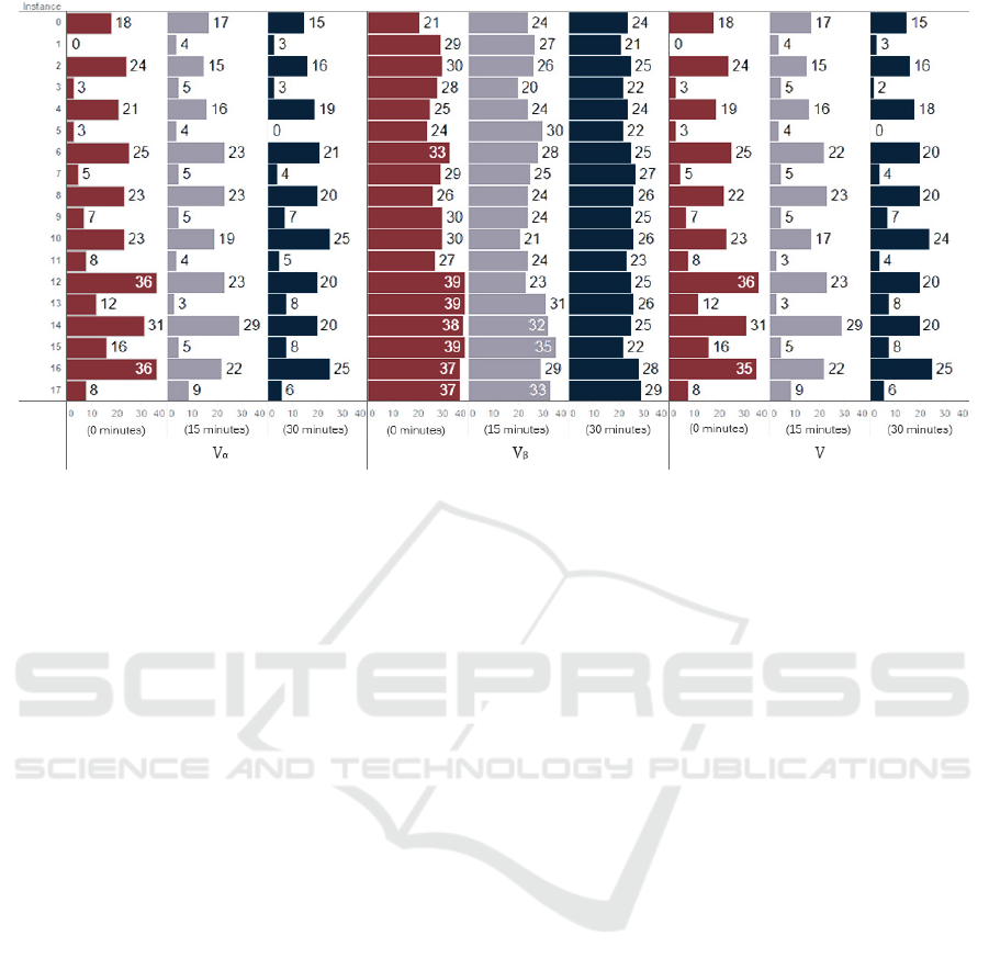
Figure 1: Number of feasible solutions got by VND with Tabu Search initialization using different services times.

jagopalan and Saydam, 2009) which introduced the

MERLP, that was used as base to the MERLP-MECC.

On our paper, whose model contains more constraints

and the instances have tights action radius, this difﬁ-

cult would naturally appear. Beside this, as we have

mentioned on previous section, the number of solu-

tions satisfying the minimum coverage constraint can

be a bottleneck for getting feasible solutions. Our in-

tuition says that maybe through a strongest penalty

when the minimum coverage constraint was not re-

spected this problem could be solved. This hypothesis

is a point to be tested on future works.

We highlight however that the feasibility, although

desirable, is not always mandatory for our proposes.

Almost feasible solutions could be satisfactory and

some relaxations can be adopted on real situations,

without a degradation of coverage quality, as for ex-

ample, the lowering the α or β values, to adapt to

some less probable scenarios. Some authors have

used goal programming (Saladin, 1982) and fuzzy

programming approaches (Araz et al., 2007) for deal-

ing speciﬁcally with those situations.

We have seen also that the results obtained here

were not so dependent of demand rates but, in another

hand, the service time has a big impact on solutions

quality. With the absence of these information, esti-

mates may be done based on the literature, as we did,

but if they were not near from real numbers, the efﬁ-

ciency of model to suggest a good allocation can be

strongly affected.

Another question, that was not dealt on the text,

but can be problematic is the imbalance of work-

load. The MERLP, as the MERLP-MECC, does not

make any consideration about balancing the work-

load. This could be done with additional constraints

on the model or a multi-objective approach, which

can be a good source for future researches.

Another possibility is to built new models that not

just states where police units should stay, but how

they could patrol areas close to where they were put

for optimizing some objective. Integrated models like

this, that joins a coverage and a routing problem are

still rare on the literature and can be explored starting

from good deterministic or stochastic models.

Finally, a possibly more useful and hard to accom-

plish continuation to this research would be a study of

case of implementation of this model in a city. This

last suggestion is more challenging due to the ethical

issues and bureaucracy involved.

ACKNOWLEDGEMENTS

The authors acknowledge CAPES, FAPEMIG and

GAPSO for the partial funding of the project. The ﬁrst

author worked in the project with funding of CAPES.

REFERENCES

Araz, C., Selim, H., and Ozkarahan, I. (2007). A

fuzzy multi-objective covering-based vehicle location

model for emergency services. Computers & Opera-

tions Research, 34(3):705 – 726. Logistics of Health

Care Management Part Special Issue: Logistics of

Health Care Management.

Basilico, N., Gatti, N., and Amigoni, F. (2012). Patrolling

security games: Deﬁnition and algorithms for solv-

A Hypercube Queuing Model Approach to the Police Units Allocation Problem

ing large instances with single patroller and single in-

truder. Artiﬁcial Intelligence, 184:78–123.

Cerqueira, D. (2005). O jogo dos sete mitos e a mis

eria da

seguranc¸a p

ublica no Brasil. IPEA, Rio de Janeiro.

Chaiken, J. M. and Dormont, P. (1976). A patrol car alloca-

tion model. Technical report, DTIC Document.

Chawathe, S. S. (2007). Organizing hot-spot police patrol

routes. In Intelligence and Security Informatics, 2007

IEEE, pages 79–86. IEEE.

Chen, X. (2013). Police patrol optimization with security

level functions. Systems, Man, and Cybernetics: Sys-

tems, IEEE Transactions on, 43(5):1042–1051.

Chiyoshi, F., Iannoni, A. P., and Morabito, R. (2011).

A tutorial on hypercube queueing models and some

practical applications in emergency service systems.

Pesquisa Operacional, 31(2):271–299.

Church, R. and ReVelle, C. (1974). The maximal cover-

ing location problem. Papers of the Regional Science

Association, 32(1):101–118.

Cihan, A., Zhang, Y., and Hoover, L. (2012). Police re-

sponse time to in-progress burglary a multilevel anal-

ysis. Police Quarterly, 15(3):308–327.

Coupe, R. T. and Blake, L. (2005). The effects of patrol

workloads and response strength on arrests at burglary

emergencies. Journal of Criminal Justice, 33(3):239–

255.

Curtin, K. M., Hayslett-McCall, K., and Qiu, F. (2010). De-

termining optimal police patrol areas with maximal

covering and backup covering location models. Net-

works and Spatial Economics, 10(1):125–145.

D’Amico, S. J., Wang, S.-J., Batta, R., and Rump, C. M.

(2002a). A simulated annealing approach to police

district design. Computers & Operations Research,

29(6):667–684.

D’Amico, S. J., Wang, S.-J., Batta, R., and Rump, C. M.

(2002b). A simulated annealing approach to police

district design. Computers & Operations Research,

29(6):667 – 684. Location Analysis.

Dell’Olmo, P., Ricciardi, N., and Sgalambro, A. (2014).

A multiperiod maximal covering location model for

the optimal location of intersection safety cameras on

an urban trafﬁc network. Procedia - Social and Be-

havioral Sciences, 108(0):106 – 117. Operational

Research for Development, Sustainability and Local

Economies.

orum Nacional de Seguranc¸a P

ublica (2013). 8

anu

ario

de seguranc¸a p

ublica. Technical report.

Glover, F. and Kochenberger, G. A. (2003). Handbook of

metaheuristics. Springer Science & Business Media.

Green, L. V. and Kolesar, P. J. (2004). Anniversary arti-

cle: Improving emergency responsiveness with man-

agement science. Management Science, 50(8):1001–

1014.

Jarvis, J. P. (1985). Approximating the equilibrium behavior

of multi-server loss systems. Management Science,

31(2):235–239.

Keskin, B. B., Li, S. R., Steil, D., and Spiller, S. (2012).

Analysis of an integrated maximum covering and pa-

trol routing problem. Transportation Research Part

E: Logistics and Transportation Review, 48(1):215 –

232. Select Papers from the 19th International Sym-

posium on Transportation and Trafﬁc Theory.

Larson, R. C. (1974). A hypercube queuing model for facil-

ity location and redistricting in urban emergency ser-

vices. Computers & Operations Research, 1(1):67–

95.

Larson, R. C. (1975). Approximating the performance of

urban emergency service systems. Operations Re-

search, 23(5):845–868.

Larson, R. C. and Rich, T. F. (1987). Travel-time analysis of

new york city police patrol cars. Interfaces, 17(2):15–

20.

Li, L., Jiang, Z., Duan, N., Dong, W., Hu, K., and Sun, W.

(2011). Police patrol service optimization based on

the spatial pattern of hotspots. In Service Operations,

Logistics, and Informatics (SOLI), 2011 IEEE Inter-

national Conference on, pages 45–50.

Lin, K. Y., Atkinson, M. P., Chung, T. H., and Glazebrook,

K. D. (2013). A graph patrol problem with random

attack times. Operations Research, 61(3):694–710.

Maltz, M. D. (1996). From poisson to the present: Applying

operations research to problems of crime and justice.

Journal of Quantitative Criminology, 12(1):3–61.

Mendes, N. F. M. and dos Santos, A. G. (2015). A tabu

search based heuristic for police units positioning. In

2015 Latin American Computing Conference, CLEI

2015, Arequipa, Peru, October 19-23, 2015, pages 1–

11.

Mendes, N. F. M., Santos, A. G., and Gonc¸alves, L. B.

(2014). M

etodos para o problema de posicionamento

de unidades policiais. In Anais do XVLI Simp

osio

Brasileiro de Pesquisa Operacional, XLVI SBPO,

pages 639–650.

Mladenovi

c, N. and Hansen, P. (1997). Variable neigh-

borhood search. Computers & Operations Research,

24(11):1097–1100.

Perrucci, A. (2011). Algoritmi esatti per la ricerca di strate-

gie ottime nel problema di pattugliamento con singolo

pattugliatore.

Rajagopalan, H. K. and Saydam, C. (2009). A minimum ex-

pected response model: Formulation, heuristic solu-

tion, and application. Socio-Economic Planning Sci-

ences, 43(4):253–262.

Ruan, S., Meirina, C., Yu, F., Pattipati, K. R., and Popp,

R. L. (2005). Patrolling in a stochastic environment.

Technical report, DTIC Document.

Saladin, B. A. (1982). Goal programming applied to police

patrol allocation. Journal of Operations Management,

2(4):239 – 249.

Simpson, N. and Hancock, P. (2009). Fifty years of oper-

ational research and emergency response. Journal of

the Operational Research Society, pages S126–S139.

Smith, R. D. (1961). Computer applications in police man-

power distribution. Field Service Division, Interna-

tional Association of Chiefs of Police.

Talbi, E.-G. (2009). Metaheuristics: from design to imple-

mentation, volume 74. John Wiley & Sons.

ICEIS 2016 - 18th International Conference on Enterprise Information Systems

Telep, C. W. and Weisburd, D. (2012). What is known

about the effectiveness of police practices in reduc-

ing crime and disorder? Police Quarterly, page

1098611112447611.

Vasconcelos, D. d. (2008). Gapatrol - uma abordagem evo-

lutiva para otimizac¸

ao de rotas de patrulha policial via

calibrac¸

ao de simulac¸

ao multiagens.

Waiselﬁsz, J. J. (2013). Mapa da viol

encia 2013. homic

ıdio

e juventude no brasil. Technical report, Centro

Brasileiro de Estudos Latino Americanos.

Weisburd, D. and Eck, J. E. (2004). What can police do to

reduce crime, disorder, and fear? The Annals of the

American Academy of Political and Social Science,

593(1):42–65.

Zhang, Y. and Brown, D. (2013). Police patrol districting

method and simulation evaluation using agent-based

model & gis. Security Informatics, 2:1–13.

Zhang, Y. and Brown, D. (2014a). Simulation optimization

of police patrol district design using an adjusted simu-

lated annealing approach. In Proceedings of the Sym-

posium on Theory of Modeling & Simulation - DEVS

Integrative, DEVS ’14, pages 18:1–18:8, San Diego,

CA, USA. Society for Computer Simulation Interna-

tional.

Zhang, Y. and Brown, D. (2014b). Simulation optimiza-

tion of police patrol districting plans using response

surfaces. Simulation, 90(6):687–705.

Zhang, Y., Huddleston, S. H., Brown, D. E., and Learmonth,

G. P. (2013). A comparison of evaluation methods

for police patrol district designs. In Proceedings of

the 2013 Winter Simulation Conference: Simulation:

Making Decisions in a Complex World, pages 2532–

2543. IEEE Press.

A Hypercube Queuing Model Approach to the Police Units Allocation Problem