Methods of Data Processing and Communication for a Web-based Wind
Flow Visualization
Marc Skutnik
1
, Luigi Lo Iacono
2
and Christian Neuhaus
1
1
WetterOnline GmbH, Bonn, Germany
2
Cologne University of Applied Sciences, Cologne, Germany
Keywords:
Wind Flow Visualization, Wind Fields, Data Tiles, Data Reduction, Data Compression, Difference-coding.
Abstract:
This paper presents methods for the reduction and compression of meteorological data for web-based wind
flow visualizations, which are tailored to the flow visualization technique. Flow data sets represent a large
amount of data and are therefore not well suited for mobile networks with low data throughput rates and high
latency. Using the mechanisms introduced in this paper, an efficient transfer of thinned out and compressed
data can be achieved, while keeping the accuracy of the visualized information almost at the same quality level
as for the original data.
1 INTRODUCTION
In weather forecasts, the expectable wind in its speed
and direction is an important forecast parameter.
Wind speeds and directions are therefore common el-
ements on geographical weather maps and are visual-
ized within meteorological applications in the shape
of wind barbs or flow vectors. The wind barb indi-
cates the wind direction and speed in a compact form
at a specific location on a weather map. Flow vec-
tors depict the same information as wind barbs, but
it is harder to discern the magnitude when viewing
vectors. Overall, for non-expert users it is difficult
to interpret these representations of wind flows and
they often cannot decide in which direction the wind
is blowing. Moreover, it is also difficult to get an im-
pression of how wind conditions will change during
the next hours as both representations do not change
the position of the wind elements on the map but mod-
ify their direction and speed only.
In the web, wind forecasts are most commonly
represented and transferred in form of images. These
images do not offer any interactivity, making it diffi-
cult for users to get a quick impression of wind flows.
Due to this, changes in time are not visible in a proper
way. A naive method to approach this issue is to use
video in order to play back a sequence of consecutive
weather conditions. This would, however, result in
a large amount of data required to be delivered to the
client causing high delays and costs, especially in mo-
bile contexts. Moreover, such an approach does not
improve anything on the users’ comprehension and
on the interactivity of the visualization, when it is still
based on wind barbs or flow vectors.
In order to solve this problem, a wind flow visu-
alization has been developed that improves the visu-
alization of wind flows on different zoom levels by
showing a streamlines movie illustrated by animated
particles. Such a wind flow visualization is more at-
tractive and has been designed in a distinctly interac-
tive manner. Based on wind vector fields, the devel-
oped wind flow visualization is able to render wind
flows in real-time within web browsers without the
use of plug-ins, providing the impression of a video.
Moreover, this wind flow visualization is executable
on mobile devices requiring the transfer of bare me-
teorological data only. Although this is already much
more efficient and resource saving than a video-based
approach, the involved meteorological base data is
still a large amount of data required to be transmitted
to the client. Hence, the goal of this work is to com-
press and simplify the bare wind data so as to achieve
an optimal balance between the amount of data re-
quired to be transferred and a still accurate visualiza-
tion rendered in an acceptable time frame.
The remaining of this paper is organized as fol-
lows. Section 2 provides a brief introduction on me-
teorological wind data structures in order to lay the
foundations. Section 3 discusses the related work on
reduction and compression methods in respect to me-
teorological data. In order to achieve the targeted goal
of a cost-efficient and accurate animated wind flow vi-
32
Skutnik, M., Iacono, L. and Neuhaus, C.
Methods of Data Processing and Communication for a Web-based Wind Flow Visualization.
In Proceedings of the 12th International Conference on Web Information Systems and Technologies (WEBIST 2016) - Volume 1, pages 32-41
ISBN: 978-989-758-186-1
Copyright
c
 2016 by SCITEPRESS – Science and Technology Publications, Lda. All rights reserved

sualization, a combination of distinct data processing
methods have to be applied. In Section 4 these meth-
ods for reducing and compressing the meteorological
data are described in detail. The evaluation results of
the proposed scheme are presented and discussed in
Section 5. The paper concludes by summarizing the
main achievements in Section 6.
2 FOUNDATIONS
The meteorological data have been taken from the In-
tegrated Forecast System (IFS) provided by the Eu-
ropean Centre for Medium-Range Weather Forecasts
(ECMWF, ). For the flow visualization, wind fields
at a height of 10 meters above the ground are used.
The meteorological data lie on a regular grid with a
0.125
◦
longitude by 0.125
◦
latitude resolution. Wind
fields in a forecast are available at 3-hourly intervals
and are selected for 17 discrete points in time for a
region of Europe (62
◦
north - 33.5
◦
north, 11
◦
west
- 35
◦
east) with 369 by 229 grid points as shown in
Figure 1.
...
...
y
x
369
229
-11°
62°
...
...
-12.125°
61°
Figure 1: Meteorological data represented in a regular grid.
For the projection of the meteorological data, a
rectangular projection has been used as the conver-
sion of a geographical coordinate into an image coor-
dinate is simple and the relations between the direc-
tions north-south and west-east are linear. The data is
projected on two different layers and four zoom steps
and is valid for every zoom step. The layers are avail-
able as tiled maps and can be requested as sprites.
The meteorological data has been analyzed with
a view to the data structure and exchange format re-
quired for them to be transferred to the client. One
solution is the transfer of complete vector fields. Be-
cause the wind flows are visualized in a view port,
the other solution is the transfer of tiled data. Thus
only visible data needs to be load. This data is repre-
sented in JSON format (Crockford, 2006). Each point
in time within a forecast represents a JSON object,
which additionally contains meta-data for the client
side’s processing and projection. All wind vectors
of one wind field are placed in a single linear array.
The meta-data object contains a date for each point
in time, the grid width and height, the distance be-
tween two grid points in x and y direction, a unique Id
and one reference pixel for the projection of tiled data
mapped as name/value pairs. In order to minimize the
amount of data, no position data for the projection is
transferred, but only one reference point.
The data can be requested over a REST-ful HTTP
(Tilkov et al., 2015) interface as a single file or as a
package with a defined amount of points in time and
are transferred over HTTP protocol. In addition to
HTTP compression, web caching is extremely use-
ful to improve loading time of not modified data. It
decrease HTTP traffic, lessen server workload, and
reduce the latency perceived by end users (Souders,
2007). Because HTTP runs over a TCP connection
not only the amount of data plays an crucial role, but
also especially in mobile networks the HTTP perfor-
mance. By the way how TCP estimates the capacity
of a connection leads in high latency in mobile net-
works. Each connection takes a full round-trip of la-
tency between the client and the server. Using per-
sistent connections and pipelining can reduce this la-
tency. Persistent connections allow for a reuse of con-
nections. When a client and a server have established
a TCP connection, the client can send GET requests
to the server to retrieve some resources. If the client
wants further resources from the server, they will have
to issue multiple GET requests, sequentially, on a per-
sistent TCP connection. Before the client can issue
an additional request, it has to wait for the previous
request to complete. To improve this, request pipelin-
ing allows for a parallel request processing. Conse-
quently, the client can send multiple requests simul-
taneously to the server. Following this, it will incur a
minimum of another round-trip of latency (Grigorik,
2013).
3 RELATED WORK
Methods for data compressing can be classified into
two classes. The first class includes methods for loss-
less compression, which reconstruct the original data
completely out of the compressed one. In contrast
to that, the second class contains lossy compression
Methods of Data Processing and Communication for a Web-based Wind Flow Visualization
33

methods, which can not fully reconstruct the data af-
ter being compressed. Methods of the latter class sep-
arate significant from less important information and
compress the substantial data only. Due to that, these
methods are able to achieve higher compression rates
with the disadvantage to only reach an approximation
of the original data after reconstruction.
Different lossless data compression techniques ex-
ist and are used in many applications, depending on
the resource type, such as text, images, videos and
so forth. For the compression of data in the web,
the most common compression schemes in HTTP
are GZIP (Deutsch, 1996b) and DEFLATE (Deutsch,
1996a). The compression can be selected by the
HTTP request header field Accept-Encoding (Field-
ing et al., 1999).
Data reduction methods remove a portion of data
points or combine various high spatial resolutions to
reduce the data volume. Various methods exist to
reduce the amount of data, which can be adapted
for a reduction of the available meteorological data.
In computer graphics and in meteorology, clustering
of data is one way to reduce the large amount of
data. A large number of wind vectors of the original
high-resolution wind field can be combined through a
weighted averaging into fewer wind vectors that ap-
proximately represent the wind field at a coarser reso-
lution, leading to a visualization of clustered data with
similar wind speeds and wind directions (Telea and
van Wijk, 1999), (Lodha et al., 2000), (Lazarus et al.,
2010).
Furthermore, the most intuitive and most com-
monly used approach for reducing the data is given
by uniform thinning. In this technique, data is re-
tained by systematically selecting one of every Nth
data point regardless of its relative importance. This
subsampling is referred to as non-adaptive thinning,
but it is used in many applications due to its sim-
plicity. Although straightforward and intuitive, non-
adaptive data thinning can result in a degraded fore-
cast because it does not discriminate between regions
of high and low information content. But this method
yields robust data reduction anyway. Further non-
adaptive strategies are simple thinning, which also in-
cludes random data points sampling, and subsampling
with averaging, where multiple data points are aver-
aged into a single data point (Hansen and Johnson,
2005), (Lazarus et al., 2010).
Moreover, intelligent thinning algorithms system-
atically select high regions in a wind field or high
wind vectors, which could have a strong effect on the
wind flow visualization. Low regions or wind vectors
with less information content are subsampled to re-
duce the amount of data (Ramachandran et al., 2005).
In video compression, different methods are used
for reducing data. MPEG involves techniques such
as difference coding and motion prediction, where
the similarity between consecutive frames in a video
stream is used to achieve a higher compression rate.
MPEG classifies each frame in a sequence as a cer-
tain type of frame, such as an I-frame, P-frame or
B-frame. An I-frame (Intra picture) is coded inde-
pendently without any reference to other pictures and
is always the first picture in a video sequence. A
P-frame (Predictive picture) is coded based on pre-
vious I or previous P pictures, while a B-frame (Bi-
directionally predictive pictures) is coded based on
either the next and/or the previous pictures (Reimers,
2008). In this context it is possible to use relations
between consecutive wind fields in a forecast to min-
imize the total amount of data to be compressed.
4 DATA REDUCTION AND
COMPRESSION
Compression techniques for meteorological data are
motivated by the necessity of transferring large flow
data sets over networks with low bandwidth and high
latency with the goal of producing visualizations of
the data in low-end mobile devices. This fact has mo-
tivated for reducing and compressing the meteorolog-
ical data. The aim is a combination of a lossless with a
lossy compression to reduce the meteorological data.
4.1 Thinning Procedure
The purpose of data thinning is to reduce the number
of characters used to represent meteorological data
within JSON format. In this context data thinning re-
duces the number of grid points. Some techniques
maintain a regular grid, which improve the client side
processing. For instance clustering of the meteoro-
logical data might lead to an irregular grid. In this
context, position data for the similar grid points must
be calculated for a projection on the client side. How-
ever, no position data will be transferred. Besides, a
non-linear interpolation must be performed for recon-
structing the data. The meteorological data are nei-
ther scattered or bundled nor incomplete. Therefore,
the use of random subsampling, subsampling with av-
eraging or intelligent thinning algorithms might result
in inconsistent distances between the grid points. Be-
cause of non-linear interpolation on the client side,
the reconstruction of an irregular grid is more costly
than the reconstruction of a regular grid.
Given is a discrete vector field as a set of wind
vectors. Thus a simple subsampling can be used for
WEBIST 2016 - 12th International Conference on Web Information Systems and Technologies
34

the thinning of the available meteorological data. The
aim of the reduction method is to construct a new
discrete representation of the vector field containing
fewer points. The advantage is that the spatial resolu-
tion can be reduced while a regular grid can be main-
tained. As a consequence, the geographical distance
or the pixel pitch between grid points respectively are
increased inversely proportional in x and y directions.
The more data are thinned, the more data need to be
reconstructed on the client side. Figure 2 shows the
simple thinning procedure.
{
{
0.125°
0.125°
{
0.25°
{
0.25°
...
...
y
x
Figure 2: Uniform thinning of a wind field.
The grid points (red circles) are selected in an
equidistant distance in x and y directions starting from
a reference grid point (red big circle). Unselected grid
points are subsampled. In this case, every second grid
point is selected. Thus the geographical distance in-
creases from 0.125
◦
to 0.25
◦
. For simple thinning, an
equivalent retention rate is obtained by selecting ev-
ery Nth observation in the x and y directions, whereby
a thinning factor N can be derived. This factor indi-
cates in which distance a grid point is selected in x and
y direction. In this case, the use of the simple thin-
ning can be considered as compression: missing grid
points of the thinning procedure are reconstructed on
the client side by the interpolation for a high spatial
resolution so as to create smooth curves. Thus the
meteorological data are an approximation of the orig-
inal data.
In addition to that, decimal places of the wind vec-
tors get shortened for a further reduction.
4.2 Difference Coding Procedure
The method for a temporal reduction performs a dif-
ference coding on wind fields depending on a refer-
ence wind field. In this context, each wind vector is
considered separately. For the determination of differ-
ences in wind speed and wind direction, both have to
be considered separately for each wind vector. This
difference coding is based on the transfer of refer-
ences instead of differences. Based on the differences,
it is decided whether data are transferred or not. This
follows from the fact that a wind vector field com-
pletely changes in time. Although wind vector fields
show differences in temporal direction no further ef-
ficient reduction can be achieved. Because meteoro-
logical data are transferred in a JSON format, thus it
is not possible to achieve a further reduction by trans-
ferring differences of wind vectors, because no char-
acters were effeminate to achieve a reduction.
The differences in speed are calculated by an ab-
solute speed deviation between two temporally con-
secutive wind vectors. Deviations in wind direction
are calculated by the angle between two wind vec-
tors. The first wind field in a forecast is always used as
the reference wind field, which is independent with-
out any reference to other wind fields.
If deviations between a reference wind vector and
a following wind vector are less than a defined thresh-
old for wind speed and wind direction, a reference on
this reference wind vector will be transferred instead
of the following wind vector. Furthermore, the ref-
erence wind vector is maintained and is used for the
next wind vector of the next wind field. If the devi-
ations are greater than the threshold for wind speed
and wind direction, the following wind vector will be
defined and transferred as a new reference wind vec-
tor.
The threshold for deviations in speed and direc-
tion is determined by the evaluation of the thinned
data. Any calculation of differences occurring on all
temporally consecutive wind fields always refers to
the reference wind field. Figure 3 shows the encoding
and decoding procedure on a sequence of a forecast.
In Figure 3, R represents a reference wind field
and C represents a coded wind field at a given point of
time. (a) Any wind field at a given t is coded by itself
and the reference wind field. In the same processing
step, a new reference wind field is created which is
valid for the following coding steps. (b) Only the first
reference wind field and the given coded wind fields
of this reference are transferred. (c) On the client side,
coded wind fields are decoded. The references within
a wind field are replaced by the respective wind vec-
tors of the preceding reference wind field. In the same
processing step, a new reference wind field is created
which is valid for following wind fields. The refer-
ence wind fields are always visualized.
For the transfer of a reference, the vector compo-
nents are replaced by a 0. An integer takes slightly
less memory in a JSON then a double. References
are written on the same position where the original
wind vector was placed. JSON allows the transfer of
null values, but it is more meaningful to transfer a
Methods of Data Processing and Communication for a Web-based Wind Flow Visualization
35

t
0
R
t
1
t
1
C
R
t
2
t
2
C
R
t
0
R
t
1
C
R
t
2
C
R
t
3
C
R
(a)
(c)
t
0
R
t
1
C
t
2
C
t
3
C
(b)
.....
.....
.....
t
3
t
3
C
Figure 3: Difference coding procedure: (a) encoding pro-
cedure, (b) transfer of coded meteorological data and (c)
decoding procedure.
0 to avoid errors on the client side. By that means,
the difference coding is optimized to achieve a higher
lossless compression rate due to the large number of
repeated values.
The compression rate of this method depends
on changes of the wind fields in time. An opti-
mal compression rate can be achieved by low tem-
poral changes. If large changes in time are avail-
able, a lower compression rate will occur. Due to this
method, it is possible to transfer regions in a wind
field with strong changes in time only. Thus, a higher
compression rate can be achieved.
5 EVALUATION
This section presents experimental results of the pro-
posed reduction and compression strategies, which
have been applied to the meteorological data. Table
1 lists the results of the thinning procedure and the
data compression for the grid resolutions and the gen-
erated JSON file sizes. Additionally, the sum over all
wind fields of the available point of times is listed.
The results show that the large amount of data can be
reduced in an efficient way. By shortening the dec-
imal places, data can be reduced by up to 48%. In
addition to that, by thinning and lossless data com-
pression a very high compression rate can be achieved
Table 1: Resolution and file size of reduced and compressed
wind fields with different thinning factor N.
N Grid Size
∅ File Size
[KB]
∅ GZIP
[KB]
∅
∑
17
[KB]
∅ GZIP
[KB]
Reduction
[%]
Reference 369x229 1370 373 23282 6333 -
All 369x229 716 181 12165 3071 87
2 185x115 181 51 3066 859 96
3 124x77 82 24 1378 408 98.25
4 93x58 46 15 788 261 98.88
5 75x47 31 10 531 176 99.24
.
.
.
10 38x24 8 3 142 55 99.76
for a given N.
When thinning-out with a factor of N = 3 in con-
junction with a lossless data compression, a data re-
duction of 98.25% has been achieved. Thus the me-
teorological data can be transferred as single point
of time or as package. Table 2 reflects the number
and file size of tiled meteorological data based on a
thinned wind field with N = 3.
Table 2: Tiled data based on a thinned wind field with thin-
ning factor N = 3.
Number of
Data Tiles
Tile Grid Size
∅ File Size
[Byte]
∅ GZIP
[Byte]
∅
∑
17
[Byte]
∅ GZIP
[Byte]
126 10x10 1177 643 17190 5141
54 15x15 2036 917 31567 9677
28 20x20 3451 1361 55991 15163
An appropriate number of 28 data tiles with a tile
grid size of 20x20 grid points has been exposed. Fur-
thermore, it was investigated which thinning factor
provides the most acceptable results to achieve a vi-
sualization with acceptable information. The wind
fields were evaluated in terms of an absolute mean
speed and direction deviation and in terms of a root
mean square error in vector differences between the
reference wind field and a thinned wind field for ev-
ery zoom step. Based on deviations and RMS, no
meaningful statement can be given on which thinning
factor is suitable to achieve a visualization with ac-
ceptable information. Because of this, a visual eval-
uation is required to determine a threshold for the re-
duction to reach a visualization with acceptable in-
formation for the user. In this evaluation, it was in-
vestigated from which thinning factor on differences
between the original data and thinned data are per-
ceptible. Table 3 shows the results of the statistical
evaluation summarized across all zoom steps.
Since the deviations of the thinned data across all
zoom steps showed the same results, it is possible to
use one version of a wind field for every zoom level.
The results of the thinning procedure show that the ac-
curacy of the thinned wind fields generally degrades
as more grid points are removed as expected. It has
been found that low wind vectors are more affected
by the thinning procedure in contrast to stronger wind
WEBIST 2016 - 12th International Conference on Web Information Systems and Technologies
36

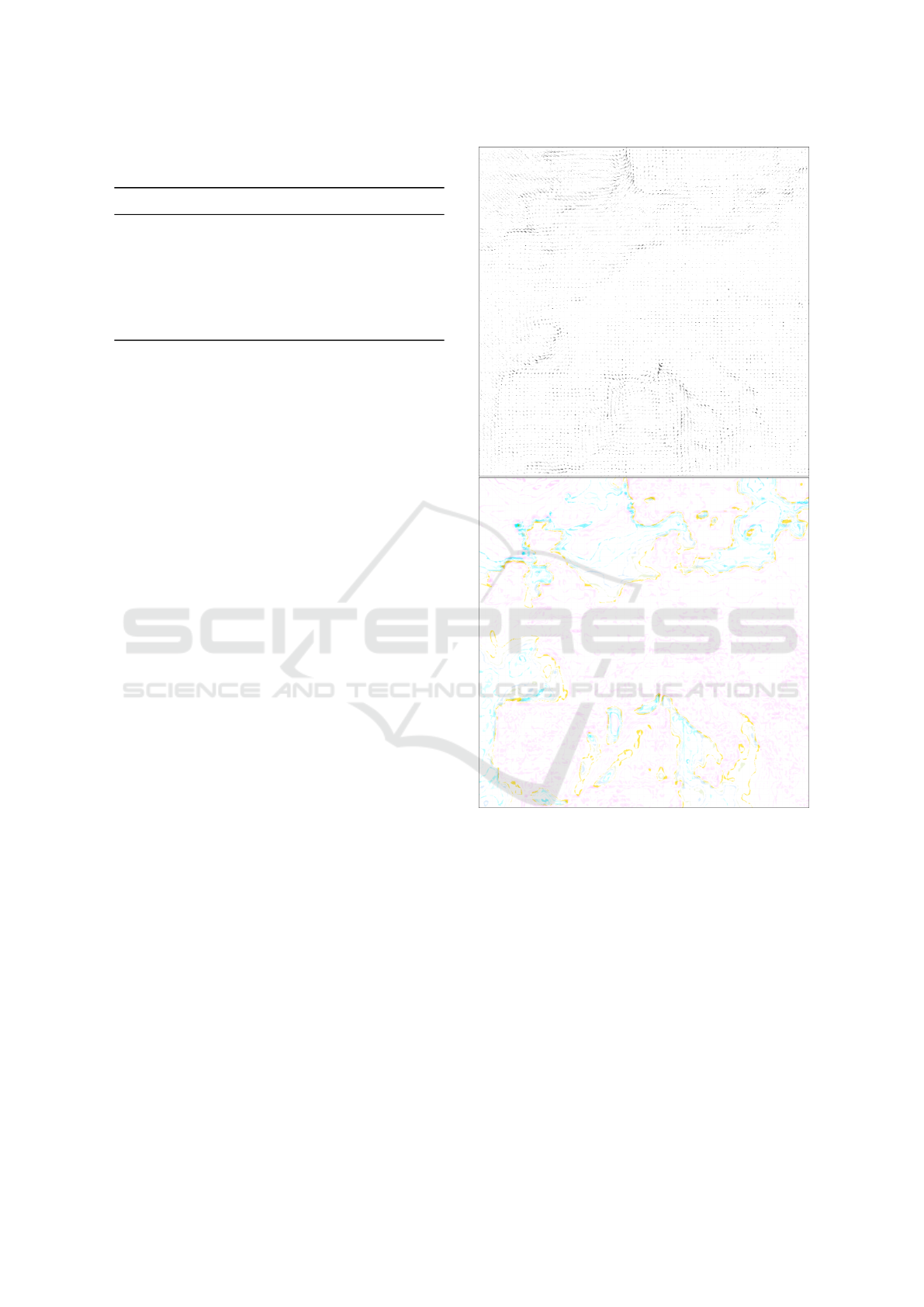
Table 3: Statistical evaluation results on deviations in speed
and direction.
N
¯
d [m/s] σ
d
[m/s]
¯
ϕ [
◦
] σ
ϕ
[
◦
] RMS
2 0.13 0.19 2.51 7.26 0.29
3 0.23 0.31 4.67 11.46 0.5
4 0.33 0.41 6.57 14.55 0.69
5 0.42 0.51 8.13 16.73 0.86
.
.
.
10 0.79 0.86 14.14 23.41 1.53
vectors, but this does not affect the visualization. Fig-
ure 4 shows difference images of thinned data in wind
directions and in wind speeds with N = 3. The results
show that strong differences of the reconstructed data
can be seen.
Although a thinning factor of N = 3 already gives
a marginal mean RMS of 0.51, the visual comparison
as given by Figure 7 between the original data and
the thinned data by N = 3 illustrates that hardly any
differences can be perceived. Only in regions with
very low wind speeds, minimum differences were per-
ceived. When using more thinned data, the results
showed more and more perceivable differences. In
comparison to that, an N = 10 gives a mean RMS of
1.54. Thus it is not possible to achieve a visualization
with acceptable accuracy.
In this case, differences are even perceived in re-
gions of strong wind speeds as shown in Figure 5. The
limit of the thinning procedure is located at a thinning
factor of N = 3 to guarantee a visualization with ac-
ceptable information.
Based on the deviations of the statistical results, a
further efficient compression can be achieved by ap-
plying difference coding to the wind fields. The pa-
rameters for the difference coding are based on the
deviations of the thinning factor of N = 3. The pa-
rameters were slightly varied to achieve an acceptable
result. A still acceptable result with the highest com-
pression can be achieved with parameters of d
u
< 0.5
m/s and wind direction deviations d
ϕ
< 10
◦
. Table 4
shows the compression results of a time series for the
given parameters wind speed deviation d
u
< 0.5 m/s
and wind direction deviation d
ϕ
< 10
◦
.
Figure 6 shows a comparison of original data on
the left side and decoded data on the right side for
t
3
. The results show that hardly any differences can
be perceived, so that a further reduction up to 50%
can be achieved while an acceptable visualization can
still be guaranteed as shown. Furthermore, the loss-
less compression in the transfer protocol can achieve
a higher mean compression rate by up to 9% for the
coded data in comparison to the original data.
Figure 4: The image on the top visualizes the differences
between the original data set and the thinned-out data set by
N = 3 in respect to the wind directions. The bottom images
visualizes the differences between the original data set and
the thinned-out data set by N = 3 in respect to the wind
speeds.
Furthermore, to determine whether acceptable
load times can be reached, the load time of the flow
visualization with meteorological data were measured
over the mobile networks 2G, 3G and 4G. To measure
the load time, three tests have been performed over a
persistent connection with pipelining. At this point,
a compromise should be found between the amount
of data to be transferred and the number of requests
the server must handle. For the first test case, the ap-
plication and unreduced data were requested. For the
second test case, the application and complete wind
Methods of Data Processing and Communication for a Web-based Wind Flow Visualization
37

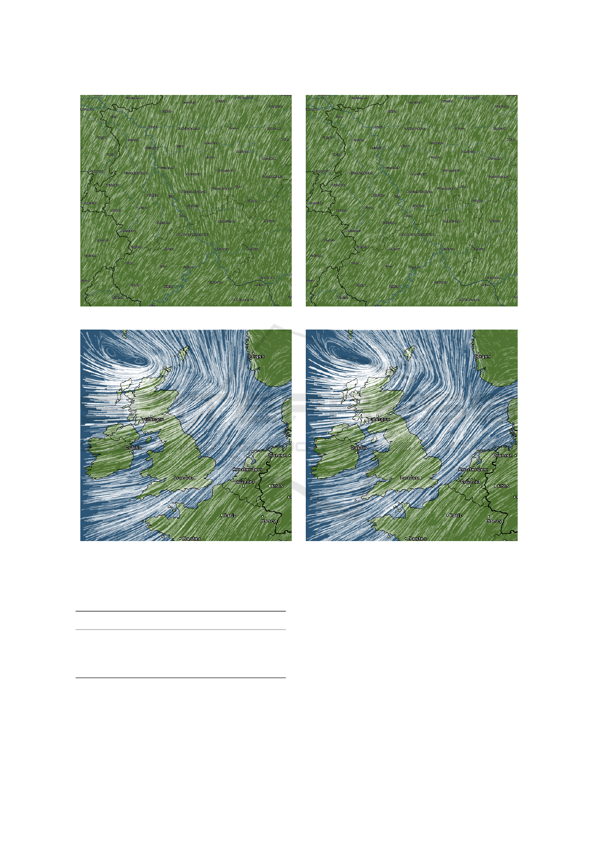
Figure 5: Comparison between original data (left) and thinned data (right) with N = 10.
Figure 6: Visual apprearance comparison between original data (left) and difference-coded wind field (right) with d
u
< 0.5 m/s
and d
ϕ
< 10
◦
.
Table 4: Data transfer volume reduction with a wind speed
deviation d
u
< 0.5 m/s and a wind direction deviation
d
ϕ
< 10
◦
.
t
File Size
[KB]
Coded
Size [KB]
Reduction
[%]
RMS
Original
GZIP [KB]
Coded
GZIP [KB]
0.5 81.4 42.8 47 0.43 24.2 4.75
1 81.4 52.6 35 0.46 24.3 11.2
1.5 81.4 50.9 37 0.54 24.1 10.8
2 81.4 56.9 30 0.45 24.3 14.1
2.5 81.4 50.4 38 0.53 24.3 10.4
3 98.8 66.2 33 0.44 34.5 19.8
fields were requested which were reduced and loss-
lessly compressed. For the third case, the application
and data tiles were requested which were reduced and
losslessly compressed. In addition, four tiled layers
were requested and a lossless compression over the
transfer protocol is performed for all test cases. Test
case one and two had to create 13 requests to load
all data for every zoom step for a) one or b) all wind
fields in a forecast. In comparison, test case three had
to create 14 requests to load all data for a map sec-
tion of every zoom step for a) one or b) all wind fields
in a forecast. In this case, two data tiles were loaded
and additionally 26 further requests would have had
to be created for the complete map section of every
zoom step. Table 5 reflects the measured load times
for each test case with 100 repeated measurements re-
WEBIST 2016 - 12th International Conference on Web Information Systems and Technologies
38

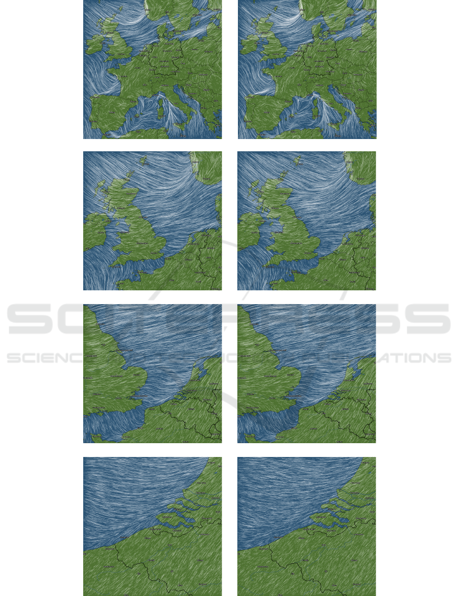
(a)
(b)
(c)
(d)
(e)
(f)
(g)
(h)
Figure 7: Comparison of original and thinned data with N = 3: (a) zoom step 0 with original data; (b) zoom step 0 with
thinned data; (c) zoom step 1 with original data; (d) zoom step 1 with thinned data; (e) zoom step 2 with original data; (f)
zoom step 2 with thinned data; (g) zoom step 3 with original data; (h) zoom step 3 with thinned data.
Methods of Data Processing and Communication for a Web-based Wind Flow Visualization
39

Table 5: Transfer times for different mobile networks.
Network
Transfer Time [s]
Test Case 1 Test Case 2 Test Case 3
a)
527 KB
b)
6487 KB
a)
178 KB
b)
562 KB
a)
156 KB
b)
184 KB
2G 29.38 405.32 11.37 33.24 11.07 15.21
3G 1.69 7.32 1.07 1.63 1.07 1.19
4G 1.49 6.77 0.88 1.45 0.88 1.01
spectively.
The results show that for test case one and gen-
erally via any 2G network, no acceptable load times
can be achieved. In comparison to that, for the test
cases two and three, acceptable load times result in a
range, which will be tolerated by the users. A study
has shown that a waiting time of approximately two
seconds is still tolerated by the users (Nah, 2004).
Moreover, the results show faster load times than the
current trend of mobile page load times of approx-
imately seven seconds (Jain and Tikir, 2013). Fur-
thermore, with the use of difference-coded data, load
times could be further improved.
6 CONCLUSION
This paper introduces the need of a wind flow visual-
ization and the associated effort of transmission over
mobile networks. The problem is addressed by the
large amount of data. The results show that it is pos-
sible to achieve a reduction of up to 98% through the
combination of lossy and lossless compressions for
a thinning factor of N = 3. It is thereby possible to
produce an almost constant visualization in compar-
ison to the original data. In this case, minimal non-
perceptible differences can occur in regions of low
wind speeds. In addition to that, a further reduction
can be reached through an appropriated threshold by
using difference coding. At this point, no general
compression rate can be specified, because difference
coding depends on changes in time. In context of
the achieved reduction, it is possible to transfer me-
teorological data within acceptable times over mobile
networks. Thus users get a fast first impression of
the wind flow visualization. In summary, it is recom-
mended to reduce the data with an N = 3 and to use
tiled data with difference-coded wind fields for the
transfer over mobile networks because of the reduced
amount of data to be transferred. For a desktop appli-
cation, a higher spatial resolution can be used and data
can be transferred as complete wind fields. Moreover,
in future a performance analysis of HTTP/2.0 in mo-
bile networks might be a treated topic, which unlike
operates much better than HTTP/1.1 (de Saxce et al.,
2015).
REFERENCES
Crockford, D. (2006). The application/json media type for
javascript object notation (json). IETF, RFC 4627.
de Saxce, H., Oprescu, I., and Chen, Y. (2015). Is http/2
really faster than http/1.1? In Computer Communica-
tions Workshops (INFOCOM WKSHPS), 2015 IEEE
Conference on, pages 293–299. IEEE.
Deutsch, L. P. (1996a). Deflate compressed data format
specification version 1.3.
Deutsch, L. P. (1996b). Gzip file format specification ver-
sion 4.3.
ECMWF. Dataset I-i Atmospheric fields - high-
reso lution forecast. http://www.ecmwf.int/en/
forecasts/datasets/set-i. Last accessed: 10.10.2015.
Fielding, R., Gettys, J., Mogul, J., Frystyk, H., Masinter,
L., Leach, P., and Berners-Lee, T. (1999). Hypertext
Transfer Protocol–HTTP/1.1.
Grigorik, I. (2013). High Performance Browser Network-
ing: What every web developer should know about
networking and web performance. O’Reilly Media.
Hansen, C. D. and Johnson, C. R. (2005). The visualization
handbook. Academic Press.
Jain, A. and Tikir, M. M. (2013). Is the web getting
faster? http://analytics.blogspot.de/2013/04/is-web-
getting-faster.html. Last accessed: January 12, 2015.
Lazarus, S. M., Splitt, M. E., Lueken, M. D., Ramachan-
dran, R., Li, X., Movva, S., Graves, S. J., and Za-
vodsky, B. T. (2010). Evaluation of data reduction
algorithms for real-time analysis. Weather and Fore-
casting, 25(3):837–851.
Lodha, S. K., Renteria, J. C., and Roskin, K. M. (2000).
Topology preserving compression of 2d vector fields.
In Visualization 2000. Proceedings, pages 343–350.
IEEE.
Nah, F. F.-H. (2004). A study on tolerable waiting time:
how long are web users willing to wait? Behaviour &
Information Technology, 23(3):153–163.
Ramachandran, R., Li, X., Movva, S., Graves, S., Greco,
S., Emmitt, D., Terry, J., and Atlas, R. (2005). Intelli-
gent data thinning algorithm for earth system numeri-
WEBIST 2016 - 12th International Conference on Web Information Systems and Technologies
40

cal model research and application. In Proc. 21st Intl.
Conf. on IIPS.
Reimers, U. (2008). DVB-Digitale Fernsehtechnik:
Datenkompression und
¨
Ubertragung. Springer-
Verlag.
Souders, S. (2007). High Performance Web Sites: Essential
Knowledge for Front-end Engineers. O’Reilly Media.
Telea, A. and van Wijk, J. J. (1999). Simplified representa-
tion of vector fields. In Proceedings of the conference
on Visualization’99: celebrating ten years, pages 35–
42. IEEE Computer Society Press.
Tilkov, S., Eigenbrodt, M., Schreier, S., and Wolf, O.
(2015). REST und HTTP: Entwicklung und Integra-
tion nach dem Architekturstil des Web (German Edi-
tion). dpunkt.verlag.
Methods of Data Processing and Communication for a Web-based Wind Flow Visualization
41