
3D Building Reconstruction using Stereo Camera and Edge Detection
Konstantinos Bacharidis
1
, Lemonia Ragia
2
, Marios Politis
1
,
Konstantia Moirogiorgou
1
and Michalis Zervakis
1
1
School of Electronic and Computer Engineering, Technical University of Crete, Kounoupidiana, Chania, Greece
2
School of Environmental Engineering, Technical University of Crete, Kounoupidiana,Chania, Greece
Keywords: Surveying, 3D Building Reconstruction, Stereo Camera Geometry, Image Processing, Edge Detection.
Abstract: Three dimensional geo-referenced data for buildings are very important for many applications like cadastre,
urban and regional planning, environmental issues, archaeology, architecture, tourism and energy. The
acquisition and update of existing databases is time consuming and involves specialized equipment and heavy
post processing of the raw data. In this study we propose a system for urban area data based on stereo cameras
for the reconstruction of the 3D space and subsequent matching with limited geodetic measurements. The
proposed stereo system along with image processing algorithms for edge detection and characteristic point
matching in the two cameras allows for the reconstruction of the 3D scene in camera coordinates. The
matching with the available geodetic data allows for the mapping of the entire scene on the word coordinates
and the reconstruction of real world distance and angle measurements.
1 INTRODUCTION
3D spatial data of buildings are very important in
recent years for many different applications. In the
cadastre and cartography domain, 3D reconstruction
of buildings has become a valuable task. For some it
is essential to obtain data of mainly handmade
objects, such as in environmental management, urban
and regional planning, population urbanization,
infrastructure, energy, archaeology communication
and tourism need the data of cities. More important,
managers and city planners must have historical and
updated object/building data at the same time.
A very simple method to acquire building data is
the computer-aided manual surveying using an
electronic distancing meter (Petzold et al., 2004). In
this method only distances between two surfaces can
be measured. Buildings data have been traditionally
acquired with geodetic techniques using the special
equipment such as total station. The reflectorless
tacheometry is a method based on measuring of
geometric dimensions. Although this method is
widely used, well established and proved to be
accurate, it does have some important disadvantages
(Petzold et al., 2004) and every point being measured
must be visible from the total station. Laser-scanning
is based on measuring distances across every pointing
direction to create the point cloud. This method
rapidly captures shapes of buildings with high
resolution, but its basic disadvantage is the heavy
post-processing of results. Photogrammetry is a well-
established method and aerial images have been
excessively used for 3D building reconstruction
(Gülch et al., 1998) (Fischer et al., 1998). An
approach that characterizes a large number of
methodologies and techniques for 3D automatic
reconstruction of buildings is given by Haala and
Kada (Haala and Kada 2010). This study verifies the
difficulties to automatically interpret 3D city models
to systems without manual intervention. In recent
years the detection and reconstruction of 3D
geometric model of an urban area with complex
buildings is based on aerial LIDAR (Light Detection
and Ranging) data (Brenner, 2005) (Elaksher and
Bethel, 2002).
In order to deal with inefficiencies of individual
modalities of data acquisition, several studies explore
the combination of sources. A 3D building
reconstruction method that integrates the aerial image
analysis with information from large-scale 2D
Geographic Information System (GIS) databases and
domain knowledge is described by Suveg and
Vosselman (Suveg and Vosselman, 2004). The use of
aerial images and the exploitation from existing 2D
GIS data is also presented (Pasko and Gruber, 1996).
The idea for using geodetic techniques combined with
Bacharidis, K., Ragia, L., Politis, M., Moirogiorgou, K. and Zervakis, M.
3D Building Reconstruction using Stereo Camera and Edge Detection.
DOI: 10.5220/0005852707150724
In Proceedings of the 11th Joint Conference on Computer Vision, Imaging and Computer Graphics Theory and Applications (VISIGRAPP 2016) - Volume 4: VISAPP, pages 715-724
ISBN: 978-989-758-175-5
Copyright
c
2016 by SCITEPRESS – Science and Technology Publications, Lda. All rights reserved
715

images of uncalibrated camera of historic buildings
for restoration in archeology is explored in (Ragia et
al., 2015). The idea of using images from Flickr and
Picasa to build accurate 3D models for archaeological
monuments is presented in (Hadjiprocopis et al.,
2014). Especially in the archaeology another
approach depicts a 5D multimedia digital model using
the 3D model in different time frames (Doulamis et
al., 2015). 3D reconstruction from a single image
combined with geometrical and topological
constraints is further discussed in (Verma et al.,
2006).
The method we develop in this paper is towards
semi-automatic 3D reconstruction of a building with
the geo reference. Although there are a lot of semi-
automatic systems for building data acquisition, there
are still open problems concerning data gathering,
database update and maintain and management of the
spatial data. Data sharing and reusing of available
spatial information is not always useful because of the
alteration or different interpretation of data. In many
spatial databases there are inconsistencies about the
location of the buildings. Some objects are
represented discrete, other appear as lists of
individual points on the ground and for some other
datasets there is a lack of information about the
thematic area.
A list of the main reasons for inadequate or
incomplete building data where additional
information is needed includes the following.
• Planners who are interested in the traffic system
measure only the façade of buildings while the
engineers who work for cadastre are interested in
acquiring the whole parcels, the buildings and all
other objects included in a private parcel like
garage and place for sport activities.
• For regional and urban planners the surveying of
geometric data plays a dominant role and before
modelling or making any decision buildings must
be surveyed, in whole or in part of the scene.
• For architectural applications, in many cases the
data of the outside of building are available but the
architects are interested only in the inside part of
the building.
• Maintenance, renovation and change of the usage
of a building needs complete 3D reconstruction of
a building and sometimes additional geometric
information in a bigger scale is required.
• Buildings with extensive alteration need an
extensive mapping from many views and for
many detailed parts.
• Environmental problems on coastal areas like
flooding, dampness and subsidence can create
structural damage of the buildings and new data
have to be acquired.
• Different interpretation by the surveyor generate
different plans, especially with buildings
constructed in an unusual way.
• Restoration of historical building needs an
extensive data acquisition of all elements.
• Some errors in the existing data may exist; some
measurements may be random.
The proposed approach is an attempt to
automatically derive the structural and
dimensionality information of a building structure
through the matching of its 3D reconstructed
coordinates with the real world coordinate system.
The building’s structural information extracted via
image contour estimation techniques provides the
points belonging to its skeleton and specifies distance
measures that can be specified in actual word
dimensions.
The paper is organized as follows. Section 2
describes the stereo layout approach with its
characteristics, advantages and limitations for 3D
reconstruction of the viewed scene. Moreover, the
relation between the 3D metric coordinate system and
the 3D physical world system is defined. A discussion
on structural information loss due to 3D
reconstruction issues along with proposed solutions is
presented in Section 3. Finally, the experimental
system layout and results are presented in Section 4.
2 STEREO LAYOUT
AND 3D RECONSTRUCTION
2.1 Camera Layout & Coordinate
System Relations
The key concept for a successful 3D reconstruction of
a scene is the derivation of the scene’s depth
information. To achieve this target a stereo camera
layout can be used, which provides the required
relation between the 3D world and 2D coordinate
systems allowing the estimation of depth information
for the viewing scene.
In order to derive the depth information we need
to estimate the parameters expressing the relation
between the physical and the image plane systems.
Essentially, what we need to estimate is first the
relation between the 3D world and the 3D camera
systems and then, the mapping parameters between
the 3D camera and the 2D image plane coordinate
systems. The first set, referred to as extrinsic
parameters, consists of the estimation of a Rotation
RGB-SpectralImaging 2016 - Special Session on RBG and Spectral Imaging for Civil/Survey Engineering, Cultural, Environmental,
Industrial Applications
716
matrix and a translation vector, whereas the latter,
referred to as intrinsic parameters, requires the
estimation of the internal camera characteristics such
as the focal length. The overall relation between the
world and image coordinate systems is expressed as:
w
xPX=⋅
(1)
with
()
,,,1
T
ii
xxyd=
being the homogenous image
coordinates with d denoting the disparity and
()
,,,1
wwww
Xxyz=
being the homogeneous 3D
world coordinates of the point
w
X
. The operator P
denotes the projection matrix containing the
extrinsic and intrinsic parameters describing the
relation between the coordinate systems:
[]
|
1
o
o
fx
PfyRT
=⋅
where [R | T] is a matrix denoting the extrinsic
parameters of the system, f denoting the camera’s
focal length and (x
o
, y
o
) being the centre coordinates
of the recorder picture, defining the intrinsic
characteristics.
The stereo layout for each camera and a 3D world
point based on eq. (1) defines the following relations
for the two (right and left) cameras:
and
left left w right right w
xPX x PX=⋅ = ⋅
(2)
All parameters required for the relation derivation
can be estimated either by using a camera calibration
process (Zhang, 2000) or an uncalibrated approach
(Hartley and Zisserman, 2003), (Hartley, 1997),
where the projection matrices are estimated through
point correspondences. The first approach provides
more accurate estimates but is more complicated,
whereas the second is simple and exploits known
reference points but it may fail in cases whether not
significant variations exist between the images of the
two cameras.
In the proposed approach we adopt the calibrated
methodology, since the appropriate estimation of both
intrinsic and extrinsic system parameters lead to more
accurate 3D reconstructions. More specifically, these
calibrated parameters allow to efficiently reverse
distortions introduced during the recording and
mapping processes. The calibration is performed
through the use of a planar surface, such as a
chessboard, which serves as a reference coordinate
system. The mapping process aims to assign the
camera centers to the reference coordinate system by
estimating the rotation and translation that minimizes
the squared distances (Zhang, 2000) between the
point correspondences using the direct linear
transformation (DLT) algorithm (Bouguet, 2013).
The estimation complexity is further increased
depending on the stereo layout used, i.e. a non-
convergent/parallel layout or a convergent one with
the camera pair being rotated at a certain angle (see
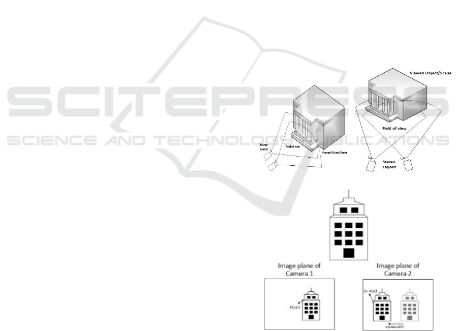
Fig 1.a, b). The simplest case used at the feasibility
study of the proposed method is the parallel stereo
layout. In such cases, the common image regions
depicted at each image plane are associated through
only a translation shift in the x-axis. By performing
a matching process, through either the use of simple
block matching methods (e.g. (Karathanasis et al.,
1996), (Zhang, 2001) or more elaborate ones such as
variational approaches (e.g. (Rallim, 2011), we can
estimate this translation map known as disparity map.
The disparity refers to the distance between two
corresponding points in the left and right image stereo
pair (see Fig 1.c):
( , ) ( , )
left i i right i i
xxyxxdy=+
(3)
with d being the disparity estimate.
(a) (b)
(c)
Figure 1: Camera Layouts and image plane relation, (a)
Non-convergent/parallel layout, adopted in our approach,
(b) convergent layout and (c) the relation between the image
planes, each viewed region scene on the left image plane is
shifted in the right plane.
3D Building Reconstruction using Stereo Camera and Edge Detection
717

2.2 3D Reconstruction of the Scene
For each point correspondence
left right
x
x↔
the
relation between them and the corresponding 3D
world point
w
X
is expressed through the relations
presented in eq. (2). In order to estimate the depicted
world point we must combine the projection matrices
and incorporate the restrictions between camera and
world points, such as the epipolar constraint. The
method of estimating the corresponding 3D world
point relating two image plane correspondences is
known as triangulation (Hartley and Zisserman,
2003) (see Fig. 2.c). Using the relations presented in
eq. (2) and eq. (3) the homogeneous DLT method (4)
can be applied leading to a linear system
representation of the form
0
w
AX⋅=
, whose solution
leads to the estimation of the 3D world point
w
X
. The
matrix A contains the projection relations between the
points and the corresponding world point and is
defined as:
3 1
3 2
3 1
3 2
'
'
TT
left left
TT
left left
TT
right right
TT
right right
xp p
yp p
A
xp p
yp p
⋅−
⋅−
=
⋅−
⋅−
with
,
ii
left right
p
p
being the i- th row vector of the
projection matrices
,
left right
P
P
for the points
() ( )
,, ','
left right
x
x
y
xx
y
==
respectively.
The vector corresponding to the world point is
found through the singular value decomposition
(SVD) factorization of the matrix A as UDV
T
, where
U and V are orthogonal matrices and D is a diagonal
matrix with non-negative entries. The unit singular
vector corresponding to the smallest singular value
provides the solution for the 3D world point
w
X
(Hartley and Zisserman, 2003).
This transformation process allows the estimation
of depth information leading to an appropriate
reconstruction of the viewing scene. However, the 3D
world system does not correspond with the actual 3D
world coordinates of the viewing scene. Information
about the scene’s longitude or latitude cannot be
estimated from the stereo layout, e.g. the building’s
width cannot be estimated. In order to do further
knowledge of the viewing scene is required.
For this task we can effectively utilize the
geographical coordinates of known points of the
building, as derived from the use of specialized geo-
reference systems, such as GPS, in combination with
the coordinates estimated from image processing, as
to estimate the missing information. For example, in
the derivation of a building’s contour, we could use
the adjacent point relation in world coordinates in the
form of width or height, to estimate the missing
dimensions of the building. Besides this use,
available points with their world coordinates can be
used as validation for the depth estimation accuracy
or as a means of refining the depth estimate during the
depth estimation process.
2.3 Combining Geo-referencing with
3D Reconstruction
We mentioned earlier that the 3D reconstructed
building can be associated with geo-referenced points
to allow the derivation of the missing dimensionality
information of the structure. This task is essentially a
new mapping process between the estimated metric
3D coordinate system and the 3D physical world
coordinate system. The transformation relation
between these systems is of the form:
Gw w
XRXT
λ
=⋅+
(4)
with
()
,y ,z
T
Gw Gw Gw Gw
Xx=
is the 3D world geo-
referenced ground point,
()
,y ,z
T
wwww
Xx=
is the
3D metric world coordinate system, λ is the
transformation parameter and R, T are the rotation
matrix and translation vector required to relate the
coordinate systems.
Given points with known geo-reference
coordinates (at least 8 points), we can estimate the
transformation parameters (λ, R, T) using a least-
squares minimization scheme. The estimated
transformation parameters enable to relate every 3D
metric on the reconstructed points to the
corresponding physical world 3D coordinates.
We can use these transformations to estimate the
3D physical coordinates of the building, or to
compute its structural dimensionality information
(width, height, volume). To speed up the estimation
process we isolate the buildings morphological
structure through image processing by extracting its
contour. We can then estimate the 3D physical
coordinates of the points belonging to the building’s
contour and thus, acquiring all the information
needed for estimating the building’s real world
structural morphology. In the following section we
present the method utilized for the extraction of the
building’s contour information using image
processing.
RGB-SpectralImaging 2016 - Special Session on RBG and Spectral Imaging for Civil/Survey Engineering, Cultural, Environmental,
Industrial Applications
718

Expanding the geo-referenced points’ (GPs) role
in the stereo rig, we can skip the utilization of a
reference system in the calibration process
(chessboard pattern). Instead, if an appropriate
number of GPs is known satisfying the requirements
that a) the corresponding points are visible on the
camera planes and b) the geo-referencing is accurate,
then we can set the word coordinate system defined
by these points as our reference system. Towards this
direction we need to employ a point identification
method for locating these points in the camera images
and then use these correspondences to perform the
calibration of the stereo rig.
2.4 3D Reconstruction Ambiguity
and Limitations
The use of a parallel stereo layout, although
simplifying the depth estimation process, provides
partial reconstruction for the structure, i.e. only for
the single view of the structure facing the stereo
layout. To produce a more complete 3D
reconstruction of the entire building, we can initially
use a convergent stereo layout with the cameras being
rotated at a certain angle, thus increasing the viewing
angle of the building’s structure being recorded. The
second, more effective approach is to combine
different viewing positions of the stereo layout, map
them to the same reference system and stitch together
all 3D reconstructions of the building sides to form a
single 3D representation.
If we now consider the case where we use a
convergent layout with the cameras displaying the
viewing object at different angles the reconstruction
accuracy depends on a) whether a calibrated approach
is used or not and b) how the additional distortions
introduced by the layout formation, such as the
keystone distortion, affects the estimation accuracy.
Similar to the parallel stereo rig layout a calibrated
approach will produce more accurate estimates taking
advantage of the impact of the distortions introduced,
allowing for some cases to undo their affect, however
requiring more complicated estimation processes. An
uncalibrated convergent stereo rig, although simpler,
will be prune to projective ambiguity in the
reconstruction process. This is due to the fact that in
the uncalibrated approach the only assumption made
is that all rays back-projecting from the reconstructed
3D point must intersect the image plane leading to
dimensionality deformations in the reconstructed
object. The projective reconstruction reflects
intersection and tangency, however it fails to preserve
the angles, the relative lengths and the volume of the
3D reconstructed object. This projective
reconstruction loss does not happen in the calibrated
approach, since the estimation of the relation between
camera and world coordinate systems, as well as the
epipolar constraint relations, do not alter or deform
the viewing angle between the rays. This enables
preservation of the parallelism, volume, length ratio
as well as of the angles of the reconstructed object,
leading to a similarity reconstruction.
The reconstruction of an uncalibrated approach
can be further strengthened leading to an affine
reconstruction that preserves the volume ratios and
the parallelism of the object. Towards this direction
we can use scene constraints and conditions, such line
parallelism indicating vanishing points, which allow
the estimation of a the epipolar plane lying at infinity
passing through the two camera centers.
Closing this topic, the selection of a calibrated
approach, such as the one deployed in our proposal,
although requiring more complex transformation
systems, will lead to a more detailed reconstruction
for the viewed object/building, preserving the
structural and volumetric characteristics.
3 LINE SEGMENTS
EXTRACTION
The previous section has described the methodology
for derivation of the 3D scene information. Since the
aim of the proposed method is to extract the 3D
morphological characteristics and dimensionality
information of the building present in the viewing
scene, we need to isolate the building from the entire
scene and extract its contour and other linear
structures, so that a relation between the estimated 3D
physical coordinates of the scene and the building’s
estimated structure can be derived.
This section addresses techniques to locate and
measure straight line segments belonging to a
building’s main structure. The main idea is to locate
several straight line segments that exist in the image
edge map. It is noted that this process mainly focuses
on the extraction of line segments that lie on the
building’s main structure (along its horizontal width
and vertical height), while more complex and detailed
objects (such as bars, rails, small windows and signs,
etc.) are not taken into account in our implementation.
The basic steps of the algorithm are outlined below,
with a further explanation on the utility of each step.
• Image color segmentation through K-Means.
• Automatic image Thresholding and conversion
to binary image.
• Edge Detection
3D Building Reconstruction using Stereo Camera and Edge Detection
719
• Edge Linking
• Straight line fitting using the Hough Transform
3.1 Image Color Segmentation
Given the RGB image of the target building, we
firstly convert it to the corresponding HSV (Hue-
Value-Saturation) model and then extract only the
Hue and Value channels prior to applying our
Segmentation scheme. The method used for the color
segmentation is the K-Means Clustering (Lloyd,
1982). This iterative method is employed to partition
all of the image’s pixels p= [p
1
, p
2
… p
n
] into k
clusters C= [C
1
, C
2
… C
k
], where obviously k≤n. The
clustering is achieved through the minimization of the
following value:
i
k
i
C
i1pC
2
arg min p
μ
=∈
−
(5)
where μ
i
is the mean of the points that belong to C
i
.
As the equation above states, the K-Means
clustering method firstly calculates each pixel’s
Euclidean distance from the mean value of the cluster
it belongs to. This mean value is often called the
cluster center or the cluster centroid value. Then it
proceeds with calculating the sum of these distances
for each cluster separately and minimizing the total
distance metric for each cluster. The minimization
procedure runs iteratively (MacKay, 2003).
At the first iteration, k random pixels are assigned
as cluster means
, μ
(t=0)
=[μ
1
, μ
2
, …, μ
k
], thus creating the
initial clusters. Then, the squared distance of each
pixel from all the mean values is computed and each
pixel is enlisted to the cluster whose mean value is the
nearest. In the next step, the new mean values are
estimated from the current clusters through the
equation
:
(t)
j
i
(t 1)
i
(t)
i
j
pC
1
p
C
+
∈
μ=
The whole process terminates when the classification
of the pixels to new clusters no longer changes.
When the method is terminated, each pixel will
have obtained a label corresponding to the cluster that
has been assigned to. In this way we can segment the
image into several color-dependent clusters. In our
algorithm, we choose k=7 (number of distinctive
colors in the image) and repeat the whole process
three times to avoid local minima. The building’s
pixels will have acquired the same integer
value(label) by the segmentation technique and by
setting to 0 all the pixels’ values in the initial image
that have obtained a different label we efficiently
isolate the building. Thus, the color difference of the
building from the rest of the image’s objects is
modeled through difference in intensity of the cluster
representing the building and the rest of the clusters.
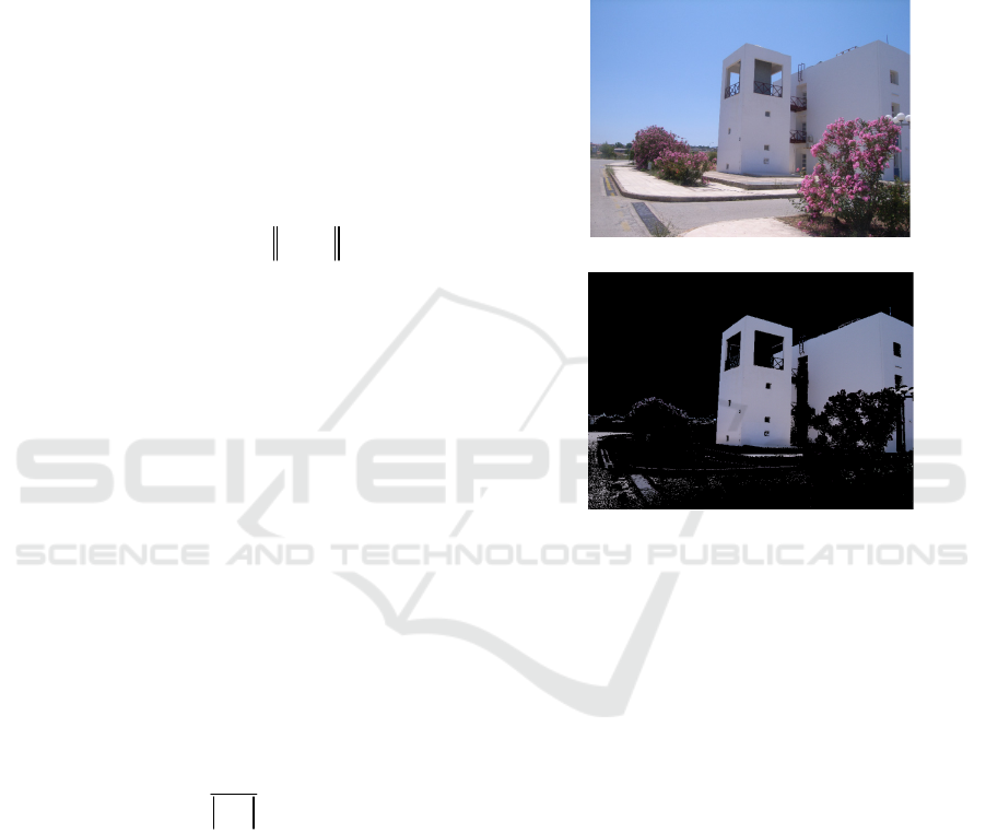
The initial RGB image as well as the image with the
isolated building are depicted in the figure below (see
Fig. 2).
(a)
(b)
Figure 2: Image color segmentation using k-means method.
(a) A picture of a building in Technical University of Crete
in its original RGB form. (b) The image of the cluster
containing the building, after the k-means method has been
applied, having isolated up to a degree the building from
other objects like vegetation, the sky etc.
3.2 Image Thresholding
In order to compute a global threshold to convert the
building-cluster image to a binary image, Otsu’s
technique is used (Otsu, 1979). This method is based
on the idea that the pixels of the image are initially
divided into various intensity levels and tries to
classify the pixels into only two regions (black and
white) as efficiently as possible with a single global
threshold. In other words, Otsu’s method criterion is
the maximization of the distinctiveness between
“light” and “dark” areas in the image. Assuming an
initial threshold value the pixels are divided into two
classes. The possibilities for a pixel p to belong to one
of the two classes are ω
1
(κ) and ω
2
(κ) and they
depend on the chosen threshold value κ, as different
κ values will result in different pairs of classes. For L
initial intensity levels the following equations apply:
RGB-SpectralImaging 2016 - Special Session on RBG and Spectral Imaging for Civil/Survey Engineering, Cultural, Environmental,
Industrial Applications
720

12
() () 1 ωκ+ωκ=
(6)
11 2 2 L
() () () ()ωκ
μ
κ+ω κ
μ
κ=
μ
(7)
where μ
L
is the total mean value over all of the L
intensity values and μ
1
, μ
2
are the mean values of the
two classes. Moreover:
222
w1122
() () () () ()σκ=ωκσκ+ωκσκ
(8)
22 2
Lw
() ()
β
σ=σ κ+σκ
(9)
The factor σ
w
(κ)
is the intra-class standard
deviation whereas the term σ
L
is the total standard
deviation for the whole image without a threshold. As
Otsu has proved:
[]
222
Lw
2
12 1 2
() ()
() () () ()
β
σκ=σ−σ κ
=ω κω κ
μ
κ−
μ
κ
(10)
so that minimizing the intra-class standard deviation
is equivalent to maximizing σ
β
, as σ
L
remains
constant.
Specifically, for all the possible threshold values
κ
i
the algorithm computes the σ
β
2
(κ
i
) values according
to eq.(10). The optimum threshold value κ
Τ
corresponds to the minimum of all the different
σ
β
2
(κ
i
) values. Once the threshold has been computed,
we are able to effectively convert our intensity image
to a binary image.
As a last step of this stage, we remove from the
binary image all connected components that have
fewer than 5000 pixels by means of area opening, in
order to further isolate the building from various
“noisy” structures.
3.3 Edge Detection
In our implementation, the Canny method is used for
edge detection. This method is effective against noise
and is likely to detect weak edges. Its effectiveness
lies on the fact that it uses two thresholds, a low
Figure 3: Binary edge image after Canny edge detector is
applied. For viewing purposes, the edges have dilated using
a 9x9 block of 1s.
threshold to detect strong edges and a high threshold
for weak edges. The weak edges are included in the
output image only if they are connected to strong
edges. The low and high threshold values selected in
this algorithm are 0.022 and 0.126 respectively.
Moreover, the standard deviation σ of the Gaussian
filter applied by the Canny detector is 1.65. The
resulting edge map is depicted in Fig. 3.
3.4 Edge Linking
A common step after the binary edge image has been
computed is edge linking. The objective is to fill gaps
that might exist between edge segments and link edge
pixels into straight edges. The implementation is
based on the idea of indirectly connecting the
endpoints of two close edge segments by placing a
certain structuring element in between those points.
The structure used is a small disk. If the endpoints of
two edge segments are close enough to each other,
then the two disks placed at each one will overlap.
Then an image thinning follows, resulting in a line at
the overlapping point and thus linking the two
previously unlinked endpoints. In addition, if there is
no other endpoint near enough, the thinning will
result in the disk’s erosion. In our implementation, the
radius of the disk is 3 pixels.
To locate endpoints of edges we set up a lookup
table by passing all possible 3 x 3 neighborhoods to a
certain function, one at a time. This function tests
whether the center pixel of the neighborhood is an
endpoint. In order for this to happen, the center pixel
must be 1 and the number of transitions between 0
and 1 along the neighborhood’s perimeter must be
two.
Line Modelling with Hough Transform:
In order to locate straight line segments on a binary
image or an edge map, the Hough Transform
technique is employed. It is a powerful method that
finds shapes whose curve is expressed by an analytic
function, for instance, a line. A line is expressed by
the equation:
ymxc =+
(11)
However, because the m value of vertical lines is
infinity, a more convenient and computationally
reasonable approach is used (Duda and Hart, 1972).
Thus, the line is expressed in polar coordinates as:
xcos ysin
ρ
=θ+θ
(12)
where ρ is the distance from the origin of the plane to
the line and θ is the angle between the horizontal x-
3D Building Reconstruction using Stereo Camera and Edge Detection
721
axis and ρ. Following this approach, a line in the (x,
y) plane corresponds to a single point in the (θ, ρ)
plane.
In our implementation, we extract peaks with
integer values greater than the ceiling integer of the
30% of the maximum value of the accumulator
matrix. The lines illustrated in Figure 4 have θ values
in the ranges [-2˚, 5˚], [175˚, 185˚], [-70˚, -85˚], [50˚,
55˚] and [65˚, 70˚ ]. It is noted that some of the lines
illustrated are produced by merging smaller line
segments associated with the same Hough transform
bin. Merged lines shorter than 150 pixels are
discarded.
Figure 4: Lines belonging to the main structure of the target
building and detected using the Hough transform. The
yellow and red asterisks correspond to a line’s beginning
and end points respectively.
4 RESULTS AND
EXPERIMENTAL SET-UP
The proposed system consists of a stereo rig of CCD
Cameras, in a non-convergent/parallel layout
formation (see Fig 1. a) with baseline distance of 5.6
cm, simulating the human visual system layout. The
intrinsic and extrinsic parameters of the system are
computed through the multi-view calibration process
described above. The triangulation procedure
described in section 2.2 allows the 3D reconstruction
of the building, as illustrated in Fig 5.b.
In our case of study, three GP points on the
building’s rooftop (marked blue in Fig 5.a) with
known geo-referenced physical coordinates are
initially used for evaluating the physical dimensions
of depth estimates. Notice that with the addition of 8
more GPs and by solving the linear equation system
defined by the relations described in eq. (3) we end
up with the transformation parameters relating the 3D
real world coordinate system with the 3D metric
based reconstructed building system.
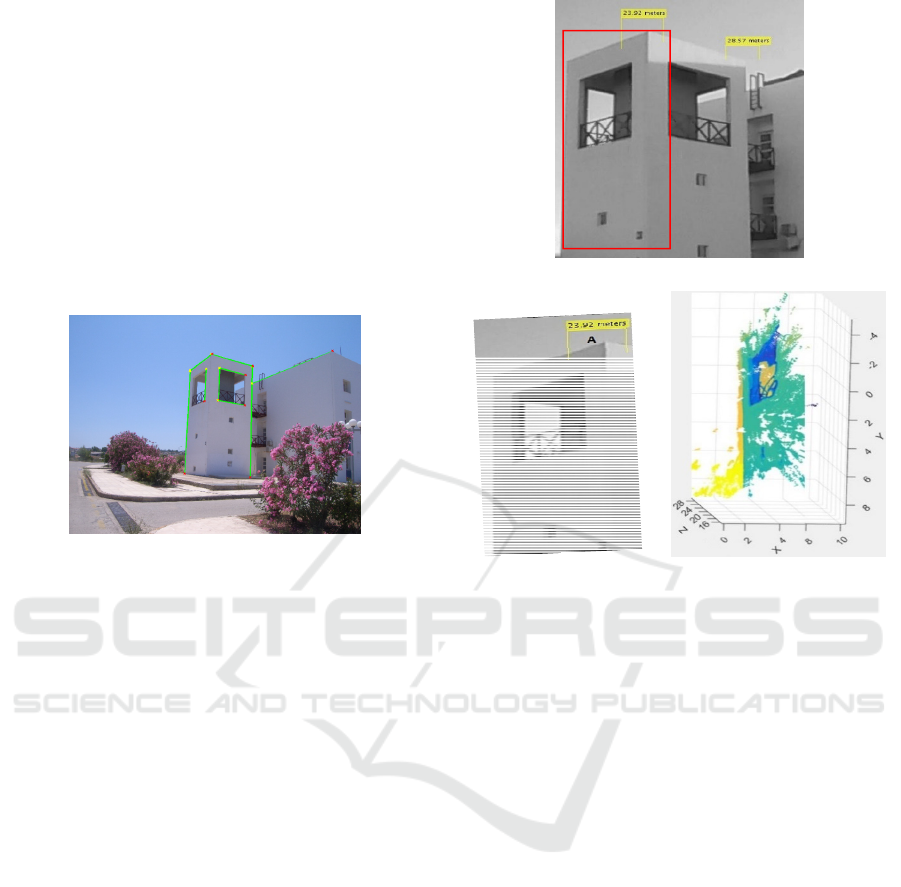
We can observe from figure 5 that the depth map
can be efficiently reconstructed, as long as we have
(a)
(b)
Figure 5: (a) The viewed scene with blue points indicating
those with known Geo-referenced coordinates used as
validation for the derived depth map and the corresponding
depth estimates (yellow boxes) based on the 3D metric
coordinates, (b) A 3D reconstruction of the left side of the
building using the triangulation approach. Different colours
indicate homogeneous regions at different depth.
many corner points available. As far as length
estimation between pairs of points of scene is
concerned, we consider the two circled corner points
of Figure 5 (a). The calibrated stereo layout leads to a
deviation error of 0.73 (5.38 – 4. 65) m or 13.57%.
We have used the known Geo-reference coordinates
of the building’s edges (blue points in Fig.5a) as a
validation for the depth estimates. The calculated
depth difference between points A and B based on our
depth estimates marked with yellow boxes in Fig 6.a
is 3.65m whereas, the corresponding difference based
on their Geo-reference coordinates is 5.38m. The
depth deviation can be further reduced with the
addition of pre-processing and post- processing steps
prior and posterior the depth derivation process.
Illumination invariance and image enhancement prior
the camera calibration stage can improve the
estimation of the stereo layout characteristics and
relations by removing shadowing and uneven
illumination or noise effects, leading eventually to
better depth estimates. As a post –processing
RGB-SpectralImaging 2016 - Special Session on RBG and Spectral Imaging for Civil/Survey Engineering, Cultural, Environmental,
Industrial Applications
722
measure, we can incorporate scene constraints and
conditions. For example, 3D line parallelism and
point intersection conditions or ground truth point
employment can serve as constraints and
homography estimation boundaries, reducing the
reconstruction ambiguity (Hartley and Zisserman,
2003).
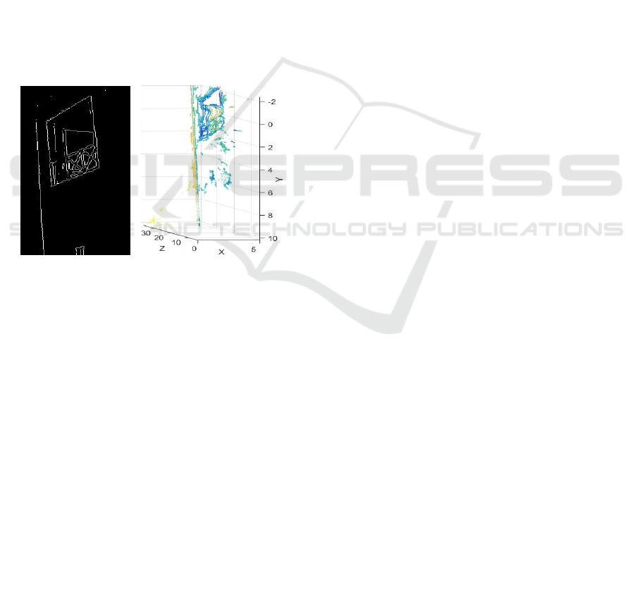
Following the proposed procedure, we extract the
building structure through the use of edge detection,
contour extraction and line structure estimation
methodology (see Fig. 6.a). We can now isolate the
points belonging to the building structure and contour
(see Fig 6.b, red box). Finally, by associating the
points belonging to the building’s contour with their
3D world coordinates, we can derive all necessary
information required to estimate the building’s real
world dimensionality (width, height and length). In
addition, using the Geo-referencing system we can
Geo-reference the building’s whole structure, its
location and volume in the real world physical
system.
(a) (b)
Figure 6: (a) Isolated structure of the building (red box)
using line segment method and (b) isolated 3D
reconstruction of the points belonging to the structure.
5 CONCLUSIONS
We propose an approach for automatic extraction the
structural and geometrical information of buildings.
The ultimate task is to provide the entire scene and its
buildings in a georeferenced form and achieve a
correspondence of its feature measurements with the
real world. The proposed approach exploits a stereo
camera system in association with appropriate image
processing tools, which enable an initial
reconstruction of the scene mapped on the camera
coordinates. Subsequently, we use a limited number
of geodetic measurements as reference in order to
map the scene onto word coordinates. An important
issue in our methodology is the successful 3D
reconstruction and the estimation of depth. Our future
aim is to further improve our estimation with the
application of pre-processing and post-processing
methodologies that will reduce both the scene and
estimation dependent deviation effects that lead to
reconstruction ambiguities. The isolation of specific
building structures from the scene can facilitate this
estimation process. Overall, it is demonstrated that
the use of stereo camera enables the relation between
the 3D georeferenced system and the camera
coordinated system, so that depth information can be
extracted.
REFERENCES
Doulamis, A., Doulamis, N., Ioannidis, C., Chrysouli, C.,
Grammalidis, N., Dimitropoulos, K., Potsiou, C.,
Stathopoulou, E., K., Ioannides, M., 2015. 5D
Modelling: An Efficient Approach for Creating
Spatiotemporal Predictive 3D Maps of Large-Scale
Cultural Resources. ISPRS Annals of Photogrammetry,
Remote Sensing and Spatial Information Sciences, 1,
pp. 61-68.
Hadjiprocopis A., Ioannides, M., Wenzel, K., Rothermel,
M., Johnsons, P., S., Fritsch, D., Doulamis, A.,
Protopapadakis, E., Kyriakaki, G., Makantasis, K.,
Weinlinger, G., Klein, M., Fellner, D., Stork, A.,
Santos, P., 2014. 4D reconstruction of the past: the
image retrieval and 3D model construction pipeline.
In Second International Conference on Remote Sensing
and Geoinformation of the Environment
(RSCy2014) International Society for Optics and
Photonics, pp. 922916-922916.
Moore, R., Lopes, J., 1999. Paper templates. In
TEMPLATE’06, 1st International Conference on
Template Production. SCITEPRESS.
Smith, J., 1998. The book, The publishing company.
London, 2
nd
edition.
Petzold, F., Bartels, H., Donath, D., 2004. New techniques
in building surveying. Proceedings of the ICCCBE-X,
pp 156.
Gülch, E., Müller, H., Labe, T. and Ragia, L., 1998. On the
performance of semi-automatic building
extraction. International Archives of Photogrammetry
and Remote Sensing, 32, pp. 331-338.
Fischer, A., Kolbe, T. H., Lang, F., Cremers, A. B.,
Förstner, W., Plümer, L. and Steinhage, V., 1998.
Extracting buildings from aerial images using
hierarchical aggregation in 2D and 3D. Computer
Vision and Image Understanding, 72(2), pp. 185-203.
Haala, N., Kada, M., 2010. An update on automatic 3D
building reconstruction. ISPRS Journal of
Photogrammetry and Remote Sensing, 65(6), pp. 570-
580.
Suveg, I., and Vosselman, G., 2004. Reconstruction of 3D
building models from aerial images and maps. ISPRS
3D Building Reconstruction using Stereo Camera and Edge Detection
723

Journal of Photogrammetry and remote sensing, 58(3),
pp. 202-224.
Pasko, M. Gruber, M., 1996. Fussion of 2D GIS Data and
aerial images for 3D building reconstruction.
International Archives of Photogrammetry and Remote
Sensing, vol. XXXI, Part B3, pp. 257-260.
Ragia, L., Sarri, F., Mania, K., 2015. 3D Reconstruction and
Visualization of Alternatives for Restoration of Historic
Buildings – A new Approach. Proceedings of the 1
st
International Conference on Geographical Information
Systems Theory, Applications and Management,
Barcelona, Spain, 28-30 April, pp. 94-102.
Brenner, C., 2005. Building reconstruction from images and
laser scanning. International Journal of Applied Earth
Observation and Geoinformation, 6(3), pp. 187-198.
Verma, V., Kumar, R. and Hsu, S., 2006. 3D building
detection and modeling from aerial LIDAR data.
In Computer Vision and Pattern Recognition, IEEE
Computer Society Conference on Vol. 2, pp. 2213-
2220.
Elaksher, A. F., and Bethel, J. S., 2002. Reconstructing 3D
buildings from LIDAR data. International Archives Of
Photogrammetry Remote Sensing and Spatial
Information Sciences, 34(3/A), pp. 102-107.
Zhang, Z., 2000. A flexible new technique for camera
calibration. IEEE Transactions on Pattern Analysis and
Machine Intelligence. vol. 22(11), pp. 1330-1334.
Hartley, R., Zisserman, A., 2003. Multiple View Geometry
in Computer Vision. Cambridge University Press.
Hartley, R., 1997. In Defense of the Eight-Point Algorithm.
IEEE® Transactions on Pattern Analysis and Machine
Intelligence, v.19 n.6.
Bouguet, J., 2013. Camera calibration toolbox for
MATLAB.
http://www.vision.caltech.edu/bouguetj/calib_doc/
Karathanasis, J., D. Kalivas, D., and J. Vlontzos, J., 1996.
Disparity estimation using block matching and dynamic
programming. IEEE Conference Electronics, Circuits
and Systems, pp.728 -731.
Zhang, L., 2001. Hierarchical block-based disparity
estimation using mean absolute difference and dynamic
programming. Proceedings International Workshop Very
Low Bit-Rate Video Coding (VLBV01), pp.114 -117.
Rallim, J., 2011. PhD thesis, Fusion and regularization of
image information in variational correspondence
methods, Universidad de Granada. Departamento de
Arquitectura y Tecnologa de Computadores,
http://hera.ugr.es/tesisugr/20702371.pdf
Lloyd, S. P. (1957). "Least square quantization in PCM".
Bell Telephone Laboratories Paper.
Lloyd., S. P. (1982). "Least squares quantization in PCM",
IEEE Transactions on Information Theory 28 (2): 129–
137.
MacKay, David (2003). "Chapter 20. An Example
Inference Task: Clustering" Information Theory,
Inference and Learning Algorithms. Cambridge
University Press. pp. 284–292.
Nobuyuki Otsu (1979). "A threshold selection method from
gray-level histograms". IEEE Trans. Sys., Man., Cyber.
9 (1): 62–66.
Duda, R. O. and P. E. Hart, "Use of the Hough
Transformation to Detect Lines and Curves in
Pictures," Comm. ACM, Vol. 15, pp. 11–15 (January,
1972)
RGB-SpectralImaging 2016 - Special Session on RBG and Spectral Imaging for Civil/Survey Engineering, Cultural, Environmental,
Industrial Applications
724
